Example - 05 - Titan Aerocapture: Part 1
In this example, you will learn to create an aerocapture feasibility chart for Titan.
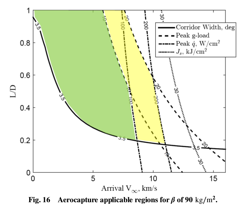
For reference, we will re-create a figure from the paper “Lu and Saikia, Feasibility Assessment of Aerocapture for Future Titan Orbiter Missions, Journal of Spacecraft and Rockets, Vol. 55, No. 5, 2018”. DOI: 10.2514/1.A34121
[3]:
from IPython.display import Image
Image(filename='../plots/lu-saikia-reference-a.png', width=400)
[3]:
We will use AMAT to recreate this figure.
[4]:
from AMAT.planet import Planet
from AMAT.vehicle import Vehicle

import numpy as np
from scipy import interpolate
import pandas as pd

import matplotlib.pyplot as plt
from matplotlib import rcParams
from matplotlib.patches import Polygon
import os
[6]:
# Create a planet object for Titan
planet=Planet("TITAN")

# Load an nominal atmospheric profile with height, temp, pressure, density data
planet.loadAtmosphereModel('../atmdata/Titan/titan-gram-avg.dat', 0 , 1 , 2, 3)

# Define the range for arrival Vinf and vehicle L/D
vinf_kms_array = np.linspace( 0.0,   16.0,  17)
LD_array       = np.linspace( 0.0,    1.0 , 11)

#vinf_kms_array = np.linspace( 0.0,   16.0,  2)
#LD_array       = np.linspace( 0.0,    1.0 , 2)
[7]:
# Create a directory to store the data.
# NOTE: You will get an error if the file already exists,
# Rename the folder to something else.

os.makedirs('../data/luSaikia2018a')

# Use a runID to prefix the files for easy access for post-processing.
runID = 'BC90RAP1700'

num_total      = len(vinf_kms_array)*len(LD_array)
count = 1

# Compute the inertial entry speed from the hyperbolic excess speed.
v0_kms_array    = np.zeros(len(vinf_kms_array))
v0_kms_array[:] = np.sqrt(1.0*(vinf_kms_array[:]*1E3)**2.0 + \
                          2*np.ones(len(vinf_kms_array))*\
                          planet.GM/(planet.RP+1000.0*1.0E3))/1.0E3

# Initialize matrices to store data.
overShootLimit_array  = np.zeros((len(v0_kms_array),len(LD_array)))
underShootLimit_array = np.zeros((len(v0_kms_array),len(LD_array)))
exitflag_os_array     = np.zeros((len(v0_kms_array),len(LD_array)))
exitflag_us_array     = np.zeros((len(v0_kms_array),len(LD_array)))
TCW_array             = np.zeros((len(v0_kms_array),len(LD_array)))
[8]:
# Compute the corridor width over the defined Vinf and L/D matrix.
# Note this will take maybe about an hour.
# If you simply want to create the plot, you can load the existing data
# in the ../data/luSaikia2018a folder as done below this cell.

for i in range(0,len(v0_kms_array)):
    for j in range(0,len(LD_array)):
        vehicle=Vehicle('Kraken', 1000.0, 90.0, LD_array[j], 3.1416, 0.0, 1.00, planet)
        vehicle.setInitialState(1000.0,0.0,0.0,v0_kms_array[i],0.0,-4.5,0.0,0.0)
        vehicle.setSolverParams(1E-5)
        overShootLimit_array[i,j],  exitflag_os_array[i,j] = \
        vehicle.findOverShootLimit (6000.0, 1.0 , -88.0, -2.0, 1E-10, 1700.0)
        underShootLimit_array[i,j], exitflag_us_array[i,j] =  \
        vehicle.findUnderShootLimit(6000.0, 1.0 , -88.0, -2.0, 1E-10, 1700.0)

        TCW_array[i,j] = overShootLimit_array[i,j] - underShootLimit_array[i,j]

        print("Run #"+str(count)+" of "+ str(num_total)+\
              ": Arrival V_infty: "+str(vinf_kms_array[i])+\
              " km/s"+", L/D:"+str(LD_array[j]) +\
              " OSL: "+str(overShootLimit_array[i,j])+\
              " USL: "+str(underShootLimit_array[i,j])+\
              ", TCW: "+str(TCW_array[i,j])+\
              " EFOS: "+str(exitflag_os_array[i,j])+\
              " EFUS: "+str(exitflag_us_array[i,j]))

        count = count +1

np.savetxt('../data/luSaikia2018a/'+runID+'vinf_kms_array.txt',vinf_kms_array)
np.savetxt('../data/luSaikia2018a/'+runID+'v0_kms_array.txt',v0_kms_array)
np.savetxt('../data/luSaikia2018a/'+runID+'LD_array.txt',LD_array)
np.savetxt('../data/luSaikia2018a/'+runID+'overShootLimit_array.txt',overShootLimit_array)
np.savetxt('../data/luSaikia2018a/'+runID+'exitflag_os_array.txt',exitflag_os_array)
np.savetxt('../data/luSaikia2018a/'+runID+'undershootLimit_array.txt',underShootLimit_array)
np.savetxt('../data/luSaikia2018a/'+runID+'exitflag_us_array.txt',exitflag_us_array)
np.savetxt('../data/luSaikia2018a/'+runID+'TCW_array.txt',TCW_array)
Run #1 of 4: Arrival V_infty: 0.0 km/s, L/D:0.0 OSL: -24.635471317420524 USL: -24.635471317420524, TCW: 0.0 EFOS: 1.0 EFUS: 1.0
Run #2 of 4: Arrival V_infty: 0.0 km/s, L/D:1.0 OSL: -23.422944245403414 USL: -27.0515137471466, TCW: 3.6285695017431863 EFOS: 1.0 EFUS: 1.0
Run #3 of 4: Arrival V_infty: 16.0 km/s, L/D:0.0 OSL: -37.36673820708165 USL: -37.36673820708165, TCW: 0.0 EFOS: 1.0 EFUS: 1.0
Run #4 of 4: Arrival V_infty: 16.0 km/s, L/D:1.0 OSL: -33.47214682791673 USL: -73.89901192915568, TCW: 40.426865101238945 EFOS: 1.0 EFUS: 1.0
Compute the deceleration and heating loads.
[9]:
acc_net_g_max_array       = np.zeros((len(v0_kms_array),len(LD_array)))
stag_pres_atm_max_array   = np.zeros((len(v0_kms_array),len(LD_array)))
q_stag_total_max_array    = np.zeros((len(v0_kms_array),len(LD_array)))
heatload_max_array        = np.zeros((len(v0_kms_array),len(LD_array)))

for i in range(0,len(v0_kms_array)):
    for j in range(0,len(LD_array)):
        vehicle=Vehicle('Kraken', 1000.0, 90.0, LD_array[j], 3.1416, 0.0, 1.00, planet)
        vehicle.setInitialState(1000.0,0.0,0.0,v0_kms_array[i],0.0,overShootLimit_array[i,j],0.0,0.0)
        vehicle.setSolverParams(1E-5)

        vehicle.propogateEntry(6000.0, 1.0, 180.0)

        # Extract and save variables to plot
        t_min_os         = vehicle.t_minc
        h_km_os          = vehicle.h_kmc
        acc_net_g_os     = vehicle.acc_net_g
        q_stag_con_os    = vehicle.q_stag_con
        q_stag_rad_os    = vehicle.q_stag_rad
        rc_os            = vehicle.rc
        vc_os            = vehicle.vc
        stag_pres_atm_os = vehicle.computeStagPres(rc_os,vc_os)/(1.01325E5)
        heatload_os      = vehicle.heatload

        vehicle=Vehicle('Kraken', 1000.0, 90.0, LD_array[j], 3.1416, 0.0, 1.00, planet)
        vehicle.setInitialState(1000.0,0.0,0.0,v0_kms_array[i],0.0,underShootLimit_array[i,j],0.0,0.0)
        vehicle.setSolverParams(1E-5)

        vehicle.propogateEntry(6000.0, 1.0, 0.0)

        # Extract and save variable to plot
        t_min_us         = vehicle.t_minc
        h_km_us          = vehicle.h_kmc
        acc_net_g_us     = vehicle.acc_net_g
        q_stag_con_us    = vehicle.q_stag_con
        q_stag_rad_us    = vehicle.q_stag_rad
        rc_us            = vehicle.rc
        vc_us            = vehicle.vc
        stag_pres_atm_us = vehicle.computeStagPres(rc_us,vc_us)/(1.01325E5)
        heatload_us      = vehicle.heatload

        q_stag_total_os  = q_stag_con_os + q_stag_rad_os
        q_stag_total_us  = q_stag_con_us + q_stag_rad_us

        acc_net_g_max_array[i,j]      = max(max(acc_net_g_os),max(acc_net_g_us))
        stag_pres_atm_max_array[i,j]  = max(max(stag_pres_atm_os),max(stag_pres_atm_os))
        q_stag_total_max_array[i,j]   = max(max(q_stag_total_os),max(q_stag_total_us))
        heatload_max_array[i,j]       = max(max(heatload_os),max(heatload_us))

        print("V_infty: "+str(vinf_kms_array[i])+" km/s"+", L/D: "+str(LD_array[j])+" G_MAX: "+str(acc_net_g_max_array[i,j])+" QDOT_MAX: "+str(q_stag_total_max_array[i,j])+" J_MAX: "+str(heatload_max_array[i,j])+" STAG. PRES: "+str(stag_pres_atm_max_array[i,j]))

np.savetxt('../data/luSaikia2018a/'+runID+'acc_net_g_max_array.txt',acc_net_g_max_array)
np.savetxt('../data/luSaikia2018a/'+runID+'stag_pres_atm_max_array.txt',stag_pres_atm_max_array)
np.savetxt('../data/luSaikia2018a/'+runID+'q_stag_total_max_array.txt',q_stag_total_max_array)
np.savetxt('../data/luSaikia2018a/'+runID+'heatload_max_array.txt',heatload_max_array)
V_infty: 0.0 km/s, L/D: 0.0 G_MAX: 0.0810485245607735 QDOT_MAX: 1.0607636054752763 J_MAX: 1020.003796275038 STAG. PRES: 0.0007204224444467468
V_infty: 0.0 km/s, L/D: 1.0 G_MAX: 0.20202892551813917 QDOT_MAX: 1.3893301148573975 J_MAX: 1252.170615904772 STAG. PRES: 0.0004253391968484517
V_infty: 16.0 km/s, L/D: 0.0 G_MAX: 17.704051243426182 QDOT_MAX: 536.4530046363565 J_MAX: 35907.65472341787 STAG. PRES: 0.15433527803169042
V_infty: 16.0 km/s, L/D: 1.0 G_MAX: 125.7389398961218 QDOT_MAX: 1065.8317771270392 J_MAX: 63948.52565398295 STAG. PRES: 0.044601211536270044
We are now ready to create the plot!
[17]:
x = np.loadtxt('../data/luSaikia2018a/'+runID+'vinf_kms_array.txt')
y = np.loadtxt('../data/luSaikia2018a/'+runID+'LD_array.txt')

Z1 = np.loadtxt('../data/luSaikia2018a/'+runID+'TCW_array.txt')
G1 = np.loadtxt('../data/luSaikia2018a/'+runID+'acc_net_g_max_array.txt')
Q1 = np.loadtxt('../data/luSaikia2018a/'+runID+'q_stag_total_max_array.txt')
H1 = np.loadtxt('../data/luSaikia2018a/'+runID+'heatload_max_array.txt')

f1 = interpolate.interp2d(x, y, np.transpose(Z1), kind='cubic')
g1 = interpolate.interp2d(x, y, np.transpose(G1), kind='cubic')
q1 = interpolate.interp2d(x, y, np.transpose(Q1), kind='cubic')
h1 = interpolate.interp2d(x, y, np.transpose(H1), kind='cubic')

x_new =  np.linspace( 0.0,   16,  170)
y_new =  np.linspace( 0.0,   1.0 ,110)
z_new =  np.zeros((len(x_new),len(y_new)))

z1_new =  np.zeros((len(x_new),len(y_new)))
g1_new =  np.zeros((len(x_new),len(y_new)))
q1_new =  np.zeros((len(x_new),len(y_new)))
h1_new =  np.zeros((len(x_new),len(y_new)))

for i in range(0,len(x_new)):
    for j in range(0,len(y_new)):

        z1_new[i,j] = f1(x_new[i],y_new[j])
        g1_new[i,j] = g1(x_new[i],y_new[j])
        q1_new[i,j] = q1(x_new[i],y_new[j])
        h1_new[i,j] = h1(x_new[i],y_new[j])

Z1 = z1_new
G1 = g1_new
Q1 = q1_new
H1 = h1_new/1000.0

X, Y = np.meshgrid(x_new, y_new)

Zlevels = np.array([2.5,3.5])
Glevels = np.array([10.0, 20.0])
Qlevels = np.array([100.0, 200.0])
Hlevels = np.array([30.0])


fig = plt.figure()
fig.set_size_inches([3.25,3.25])
plt.ion()
plt.rc('font',family='Times New Roman')
params = {'mathtext.default': 'regular' }
plt.rcParams.update(params)

ZCS1 = plt.contour(X, Y, np.transpose(Z1), levels=Zlevels, colors='black')
plt.clabel(ZCS1, inline=1, fontsize=10, colors='black',fmt='%.1f',inline_spacing=1)
ZCS1.collections[0].set_linewidths(1.50)
ZCS1.collections[1].set_linewidths(1.50)
ZCS1.collections[0].set_label(r'$TCW, deg.$')

GCS1 = plt.contour(X, Y, np.transpose(G1), levels=Glevels, colors='blue',linestyles='dashed')
plt.clabel(GCS1, inline=1, fontsize=10, colors='blue',fmt='%d',inline_spacing=0)
GCS1.collections[0].set_linewidths(1.50)
GCS1.collections[1].set_linewidths(1.50)
GCS1.collections[0].set_label(r'$g$'+r'-load')

QCS1 = plt.contour(X, Y, np.transpose(Q1), levels=Qlevels, colors='red',linestyles='dotted',zorder=11)
plt.clabel(QCS1, inline=1, fontsize=10, colors='red',fmt='%d',inline_spacing=0)
QCS1.collections[0].set_linewidths(1.50)
QCS1.collections[1].set_linewidths(1.50)
QCS1.collections[0].set_label(r'$\dot{q}$'+', '+r'$W/cm^2$')


HCS1 = plt.contour(X, Y, np.transpose(H1), levels=Hlevels, colors='xkcd:brown',linestyles='dashdot')
plt.clabel(HCS1, inline=1, fontsize=10, colors='xkcd:brown',fmt='%d',inline_spacing=0)
HCS1.collections[0].set_linewidths(1.75)
HCS1.collections[0].set_label(r'$Q$'+', '+r'$kJ/cm^2$')

plt.xlabel("Arrival "+r'$V_\infty$'+r', km/s' ,fontsize=10)
plt.ylabel("L/D",fontsize=10)
plt.xticks(fontsize=10)
plt.yticks(fontsize=10)
ax = plt.gca()
ax.tick_params(direction='in')
ax.yaxis.set_ticks_position('both')
ax.xaxis.set_ticks_position('both')
plt.legend(loc='upper right', fontsize=8)


dat0 = ZCS1.allsegs[1][0]
x1,y1=dat0[:,0],dat0[:,1]
F1 = interpolate.interp1d(x1, y1, kind='linear',fill_value='extrapolate', bounds_error=False)

dat1 = GCS1.allsegs[0][0]
x2,y2=dat1[:,0],dat1[:,1]
F2 = interpolate.interp1d(x2, y2, kind='linear',fill_value='extrapolate', bounds_error=False)

dat2 = QCS1.allsegs[0][0]
x3,y3= dat2[:,0],dat2[:,1]
F3 = interpolate.interp1d(x3, y3, kind='linear',fill_value='extrapolate', bounds_error=False)


x4 = np.linspace(0,30,301)
y4 = F1(x4)
y5 = F2(x4)
y6 = F3(x4)

y7 = np.minimum(y5,y6)

plt.fill_between(x4, y4, y7, where=y4<=y7,color='xkcd:neon green')
plt.xlim([0.0,16.0])
plt.ylim([0.0,1.0])

plt.savefig('../plots/LuSaikia2018a-fig16.png',bbox_inches='tight')
plt.savefig('../plots/LuSaikia2018a-fig16.pdf', dpi=300,bbox_inches='tight')
plt.savefig('../plots/LuSaikia2018a-fig16.eps', dpi=300,bbox_inches='tight')
The PostScript backend does not support transparency; partially transparent artists will be rendered opaque.
The PostScript backend does not support transparency; partially transparent artists will be rendered opaque.
The PostScript backend does not support transparency; partially transparent artists will be rendered opaque.
The PostScript backend does not support transparency; partially transparent artists will be rendered opaque.
[18]:
from IPython.display import Image
Image(filename='../plots/LuSaikia2018a-fig16-higher-res.png', width=400)
[18]:
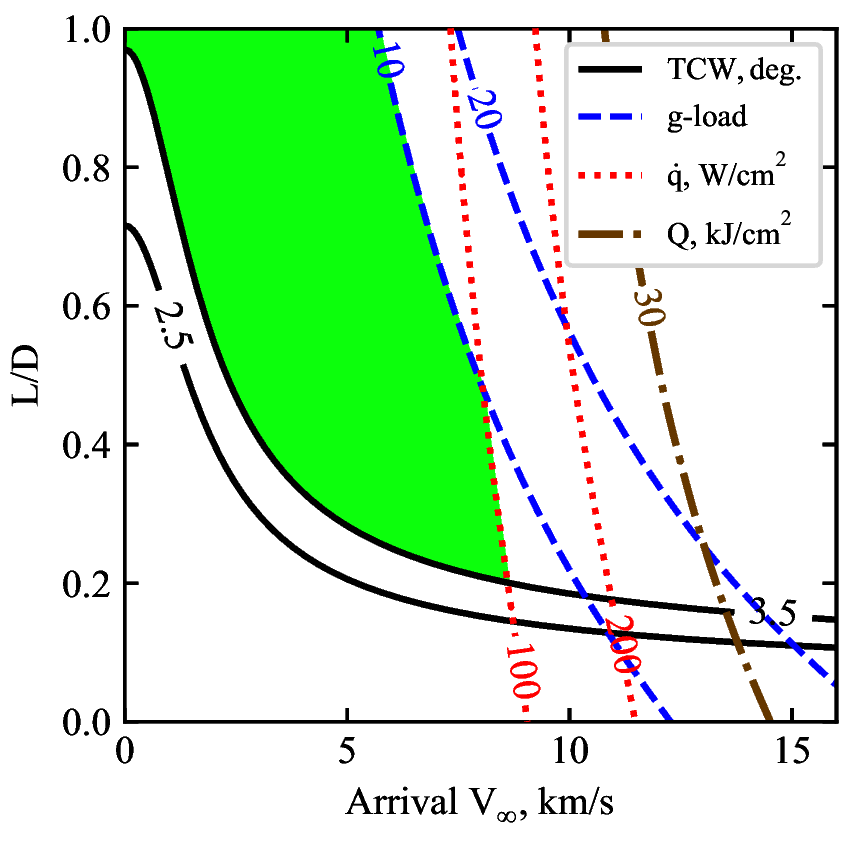
The plots are now saved in plots/LuSaikia2018a and should match with the results from the paper.
Congratulations! You have created an aerocapture feasibility chart for Titan. In the next example, you will recreate the same chart for a different vehicle ballistic coefficient.