Example - 41 - Hera - Saturn (Concept)

from AMAT.planet import Planet
from AMAT.vehicle import Vehicle

import numpy as np
import matplotlib.pyplot as plt

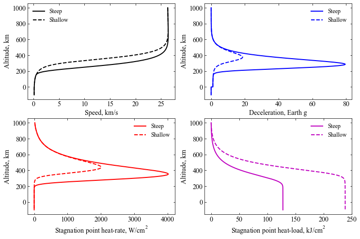
This notebook simulates the atmospheric entry of the Saturn entry probe which was part of the Hera mission concept study. http://dx.doi.org/10.1016/j.pss.2015.06.020

# Set up the planet and atmosphere model.
planet=Planet("SATURN")
planet.h_skip = 1000.0E3
planet.h_trap = -100.0E3
planet.loadAtmosphereModel('../atmdata/Saturn/saturn-nominal.dat', 0 , 1 , 2, 3, heightInKmFlag=True)

# Set up the vehicle
vehicle1=Vehicle('Hera-Saturn-Probe-steep', 220, 269, 0.0, np.pi*1.0**2.0*0.25, 0.0, 0.18, planet)
vehicle2=Vehicle('Hera-Saturn-Probe-shallow', 220, 269, 0.0, np.pi*1.0**2.0*0.25, 0.0, 0.18, planet)

# Set up entry parameters
vehicle1.setInitialState(1000.0,0.0,0.0,26.3,0.0,-22.0,0.0,0.0)
vehicle2.setInitialState(1000.0,0.0,0.0,26.3,0.0,-9.0,0.0,0.0)

# Set up solver
vehicle1.setSolverParams(1E-6)
vehicle2.setSolverParams(1E-6)

# Propogate vehicle entry trajectory
vehicle1.propogateEntry (100*60.0,0.1,0.0)
vehicle2.propogateEntry (100*60.0,0.1,0.0)

# import rcParams to set figure font type
from matplotlib import rcParams

fig = plt.figure(figsize=(12,8))
plt.rc('font',family='Times New Roman')
params = {'mathtext.default': 'regular' }
plt.rcParams.update(params)

plt.subplot(2, 2, 1)
plt.plot(vehicle1.v_kmsc, vehicle1.h_kmc, 'k-', linewidth=2.0, label='Steep')
plt.plot(vehicle2.v_kmsc, vehicle2.h_kmc, 'k--', linewidth=2.0, label='Shallow')
plt.xlabel('Speed, km/s',fontsize=14)
plt.ylabel('Altitude, km', fontsize=14)
plt.legend(loc='upper left', fontsize=12, frameon=False)
ax=plt.gca()
ax.tick_params(direction='in')
ax.yaxis.set_ticks_position('both')
ax.xaxis.set_ticks_position('both')
ax.tick_params(axis='x',labelsize=14)
ax.tick_params(axis='y',labelsize=14)

plt.subplot(2, 2, 2)
plt.plot(vehicle1.acc_net_g, vehicle1.h_kmc, 'b-', linewidth=2.0, label='Steep')
plt.plot(vehicle2.acc_net_g, vehicle2.h_kmc, 'b--', linewidth=2.0, label='Shallow')
plt.xlabel('Deceleration, Earth g',fontsize=14)
plt.ylabel('Altitude, km', fontsize=14)
plt.legend(loc='upper right', fontsize=12, frameon=False)
ax=plt.gca()
ax.tick_params(direction='in')
ax.yaxis.set_ticks_position('both')
ax.xaxis.set_ticks_position('both')
ax.tick_params(axis='x',labelsize=14)
ax.tick_params(axis='y',labelsize=14)

plt.subplot(2, 2, 3)
plt.plot(vehicle1.q_stag_total, vehicle1.h_kmc,'r-', linewidth=2.0, label='Steep')
plt.plot(vehicle2.q_stag_total, vehicle2.h_kmc,'r--', linewidth=2.0, label='Shallow')
plt.xlabel('Stagnation point heat-rate, '+r'$W/cm^2$',fontsize=14)
plt.ylabel('Altitude, km', fontsize=14)
ax=plt.gca()
plt.legend(loc='upper right', fontsize=12, frameon=False)
ax.tick_params(direction='in')
ax.yaxis.set_ticks_position('both')
ax.xaxis.set_ticks_position('both')
ax.tick_params(axis='x',labelsize=14)
ax.tick_params(axis='y',labelsize=14)


plt.subplot(2, 2, 4)
plt.plot(vehicle1.heatload/1.0E3, vehicle1.h_kmc, 'm-', linewidth=2.0, label='Steep')
plt.plot(vehicle2.heatload/1.0E3, vehicle2.h_kmc, 'm--', linewidth=2.0, label='Shallow')
plt.xlabel('Stagnation point heat-load, '+r'$kJ/cm^2$',fontsize=14)
plt.ylabel('Altitude, km', fontsize=14)
plt.legend(loc='upper right', fontsize=12, frameon=False)
ax=plt.gca()
ax.tick_params(direction='in')
ax.yaxis.set_ticks_position('both')
ax.xaxis.set_ticks_position('both')
ax.tick_params(axis='x',labelsize=14)
ax.tick_params(axis='y',labelsize=14)

plt.savefig('../plots/hera-saturn-probe.png',bbox_inches='tight')
plt.savefig('../plots/hera-saturn-probe.pdf', dpi=300,bbox_inches='tight')
plt.savefig('../plots/hera-saturn-probe.eps', dpi=300,bbox_inches='tight')

plt.show()