Example - 62 - Approach Trajectories for Two Probes at Neptune

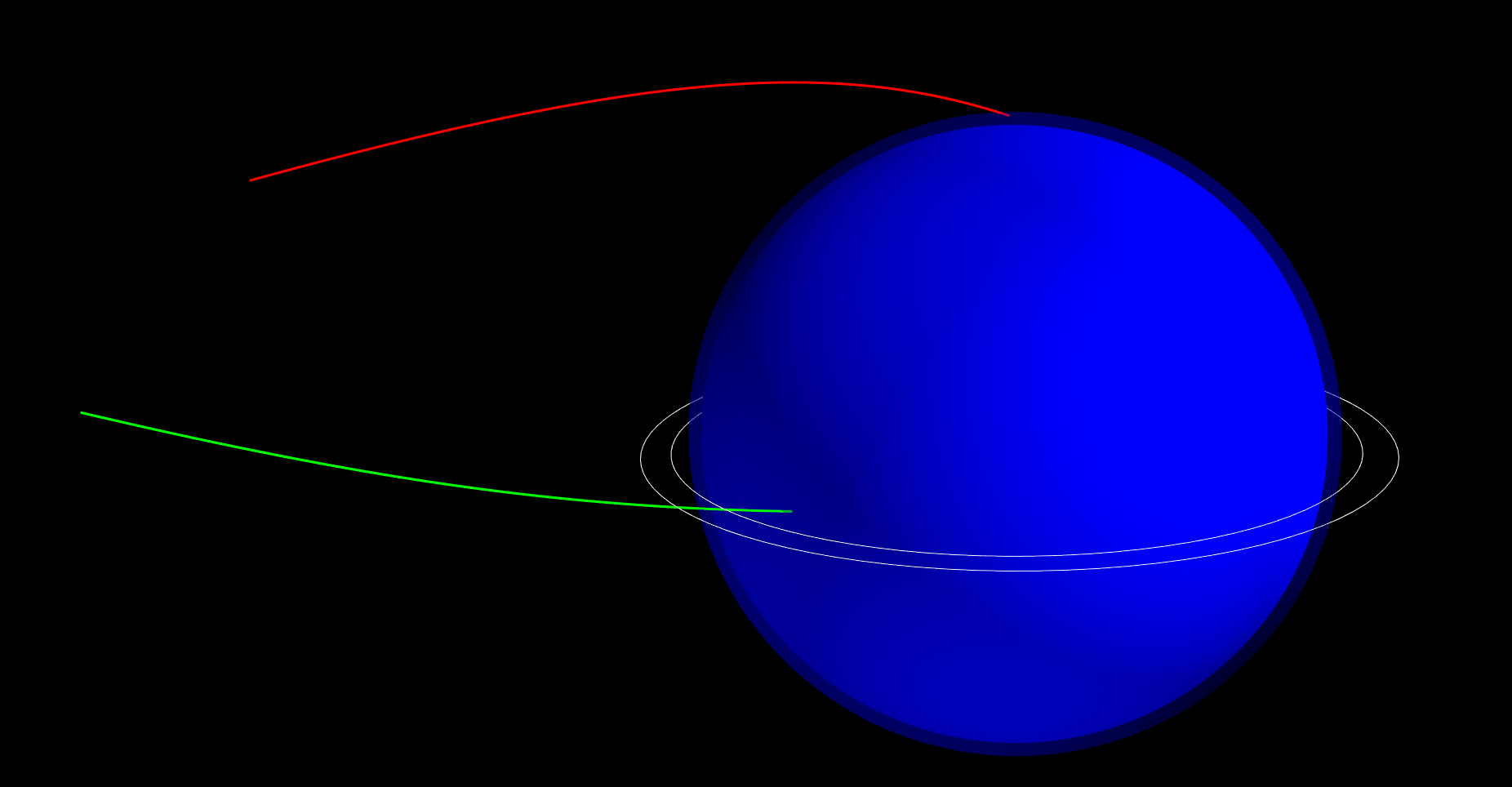
In this example, we illustrate the approach trajectories for two probes, one equatorial and one polar delivered from a single approach trajectory at Neptune.

Note: This example requires Mayavi for visualization and requires the following packages to be to be installed in your virtual env: pyqt5, vtk, mayavi.

Note: For the 3D viz, tt is recommended that you run this example by running the python file using: python example-62-two-probes-equatorial-polar.py from your virtual env terminal instead of this Jupyter Notebook. If you use this Jupyter Notebook, then you need to have the following additional packages installed ipywidgets and ipyevents, and must do jupyter nbextension install --py mayavi --user before you start the notebook.

from mayavi import mlab
mlab.init_notebook(backend='ipy')

import numpy as np

from AMAT.approach import Approach

Notebook initialized with ipy backend.

Make two probes with psi = pi [polar] and psi = 3pi/2 [equatorial, prograde]

probe1 = Approach("NEPTUNE",
                    v_inf_vec_icrf_kms=np.array([17.78952518, 8.62038536, 3.15801163]),
                    rp=(24764 + 400) * 1e3, psi=np.pi,
                    is_entrySystem=True, h_EI=1000e3)


probe2 = Approach("NEPTUNE",
                    v_inf_vec_icrf_kms=np.array([17.78952518, 8.62038536, 3.15801163]),
                    rp=(24764 + 400) * 1e3, psi=3* np.pi/2,
                    is_entrySystem=True, h_EI=1000e3)

theta_star_arr_probe1 = np.linspace(-1.8, probe1.theta_star_entry, 101)
pos_vec_bi_arr_probe1 = probe1.pos_vec_bi(theta_star_arr_probe1)/24764e3


theta_star_arr_probe2 = np.linspace(-1.8, probe2.theta_star_entry, 101)
pos_vec_bi_arr_probe2 = probe2.pos_vec_bi(theta_star_arr_probe2)/24764e3

x_arr_probe1 = pos_vec_bi_arr_probe1[0][:]
y_arr_probe1 = pos_vec_bi_arr_probe1[1][:]
z_arr_probe1 = pos_vec_bi_arr_probe1[2][:]

x_arr_probe2 = pos_vec_bi_arr_probe2[0][:]
y_arr_probe2 = pos_vec_bi_arr_probe2[1][:]
z_arr_probe2 = pos_vec_bi_arr_probe2[2][:]


u = np.linspace(0, 2 * np.pi, 100)
v = np.linspace(0, np.pi, 100)
x = 1*np.outer(np.cos(u), np.sin(v))
y = 1*np.outer(np.sin(u), np.sin(v))
z = 1*np.outer(np.ones(np.size(u)), np.cos(v))

x1 = 1.040381198513972*np.outer(np.cos(u), np.sin(v))
y1 = 1.040381198513972*np.outer(np.sin(u), np.sin(v))
z1 = 1.040381198513972*np.outer(np.ones(np.size(u)), np.cos(v))


x_ring_1 = 1.1*np.cos(u)
y_ring_1 = 1.1*np.sin(u)
z_ring_1 = 0.0*np.cos(u)

x_ring_2 = 1.2*np.cos(u)
y_ring_2 = 1.2*np.sin(u)
z_ring_2 = 0.0*np.cos(u)

mlab.figure(bgcolor=(0,0,0), size=(1200,800))
s1 = mlab.mesh(x, y, z, color=(0,0,1))
s2 = mlab.mesh(x1, y1, z1, color=(0,0,1), opacity=0.3)
r1 = mlab.plot3d(x_ring_1, y_ring_1, z_ring_1, color=(1,1,1), line_width=1, tube_radius=None)
r2 = mlab.plot3d(x_ring_2, y_ring_2, z_ring_2, color=(1,1,1), line_width=1, tube_radius=None)

p1 = mlab.plot3d(x_arr_probe1, y_arr_probe1, z_arr_probe1, color=(1,0,0), line_width=3, tube_radius=None)
p2 = mlab.plot3d(x_arr_probe2, y_arr_probe2, z_arr_probe2, color=(0,1,0), line_width=3, tube_radius=None)


mlab.show()
# uncomment the line below if running the Jupyter Notebook
# p2

Plot the approach trajectories of both probes

from IPython.display import Image
Image(filename="../plots/example-69-equatorial-polar-probe-two-probes.png", width=800)

Compute the atmosphere-relative entry conditions for both probes

Polar probe

print("Entry altitude, km: "+ str(probe1.h_EI/1e3))
print("Entry longitude BI, km: "+ str(round(probe1.longitude_entry_bi*180/np.pi, 2)))
print("Entry latitude BI, deg: "+ str(round(probe1.latitude_entry_bi*180/np.pi, 2)))
print("Atm. relative entry speed, km/s: "+str(round(probe1.v_entry_atm_mag/1e3, 4)))
print("Atm. relative heading angle, deg: "+str(round(probe1.heading_entry_atm*180/np.pi, 4)))
print("Atm. relative EFPA, deg: "+str(round(probe1.gamma_entry_atm*180/np.pi, 4)))

Entry altitude, km: 1000.0
Entry longitude BI, km: 4.25
Entry latitude BI, deg: 87.79
Atm. relative entry speed, km/s: 30.5681
Atm. relative heading angle, deg: 90.2007
Atm. relative EFPA, deg: -9.1713

Equatorial probe

print("Entry altitude, km: "+ str(probe2.h_EI/1e3))
print("Entry longitude BI, km: "+ str(round(probe2.longitude_entry_bi*180/np.pi, 2)))
print("Entry latitude BI, deg: "+ str(round(probe2.latitude_entry_bi*180/np.pi, 2)))
print("Atm. relative entry speed, km/s: "+str(round(probe2.v_entry_atm_mag/1e3, 4)))
print("Atm. relative heading angle, deg: "+str(round(probe2.heading_entry_atm*180/np.pi, 4)))
print("Atm. relative EFPA, deg: "+str(round(probe2.gamma_entry_atm*180/np.pi, 4)))

Entry altitude, km: 1000.0
Entry longitude BI, km: -74.91
Entry latitude BI, deg: 1.66
Atm. relative entry speed, km/s: 27.866
Atm. relative heading angle, deg: 13.7856
Atm. relative EFPA, deg: -10.0695