Example - 72 - Uranus Aerocapture - Part 1
In this example, we illustrate the use of AMAT for a preliminary analysis of an aerocapture mission concept to Uranus.
Ground Rules and Assumptions:
The mission must launch between 2028 and 2038, and arrive at Uranus no later than 8 years after launch.
The nominal orbiter and probe mass is 1700 kg and 300 kg respectively.
The launch vehicle should be capable of launching a spacecraft at least 4000 kg in mass, assuming 2000 kg of useful delivered mass to Uranus orbit and 2000 kg of aerocapture system mass (including propellant for any deep space manuevers).
Including 20% mass margin, the launch vehicle must have a launch capability of at least 5000 kg.
The aerocapture vehicle will have a maximum L/D of 0.36 (using an Apollo-derived aeroshell).
The mission design must allow at least 1 deg. of theoretical corridor width (TCW) at Uranus.
The maximum deceleration load is not to exceed 15g.
The maximum stagnation-point peak heat rate is not to exceed 5000 W/cm^2.
The maximum stagnation-point total heat load is not to exceed 200 kJ/cm^2.
The mission must place the orbiter into an orbit with an inclination as close to equatorial as possible.
The maximum capability launch vehicle available is the Falcon Heavy Expendable.
The initial capture orbit shall have an apoapsis altitude of 500,000 km or greater.
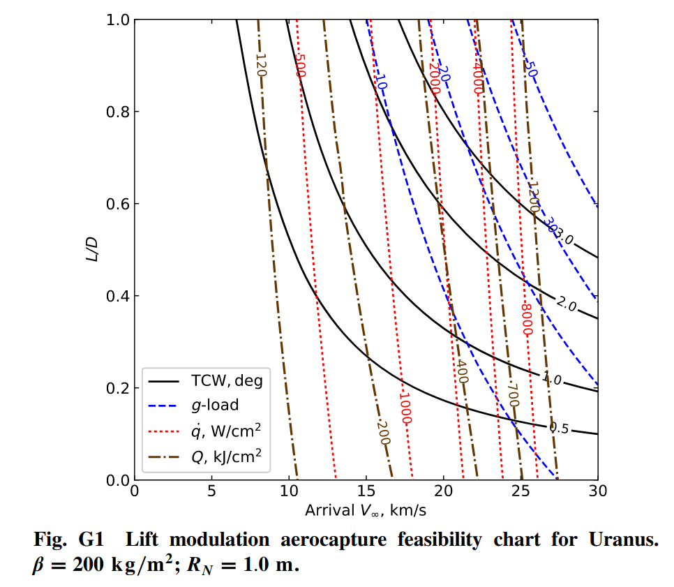
We use an existing feasibility chart from Girija et al. (2022) Girija A. P. et al. Quantitative Assessment of Aerocapture and Applications to Future Missions, Journal of Spacecraft and Rockets, 2022 for preliminary analysis.
[1]:
from IPython.display import Image
Image(filename="../plots/uranus-feasibility-chart-girija-et-al-2022.png", width=700)
[1]:
Derived Mission Requirements:
Because of the assumption #5 that the maximum allowed vehicle L/D is 0.24, and assumption #6 that a 1 deg TCW is required, we immediately see that the interplanetary trajectory arrival \(V_{\infty}\) must be at least 20 km/s. This implies a high-energy trajectory is required. Because of requirement #8 that the maximum heat rate is not to exceed 5000 \(W/cm^2\), we limit the maximum arrival \(V_{\infty}\) to 24 km/s.
Let us now look at the available high-energy trajectory options to Uranus which satisfy the above derived mission requirement. We will first look at the launch capability vs launch date chart using AMAT. Requirement #4 states that the launch capability shoud be at least 5000 kg.
[2]:
import pandas as pd
import matplotlib.pyplot as plt
[3]:
from AMAT.launcher import Launcher
from AMAT.interplanetary import Interplanetary
[4]:
interplanetary1 = Interplanetary(ID="Uranus High Energy",
                                 datafile='../interplanetary-data-private/uranus/uranus-high-energy.xlsx',
                                 sheet_name='Sheet1',
                                 Lcdate_format=None)

launcher1 = Launcher('Falcon Heavy Exp. with kick',
                     datafile='../launcher-data/falcon-heavy-expendable-w-star-48.csv')
[5]:
interplanetary1.plot_launch_mass_vs_launch_date(launcherObj=launcher1)
No artists with labels found to put in legend.  Note that artists whose label start with an underscore are ignored when legend() is called with no argument.
The PostScript backend does not support transparency; partially transparent artists will be rendered opaque.
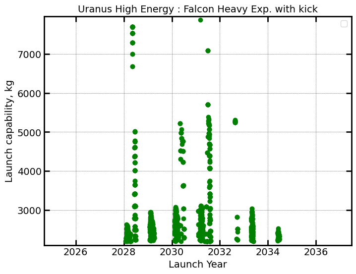
It appears that there are some trajectories which have a launch capability exceeding 5000 kg within the desired launch window. Let us now look at the trajectories with launch mass, time of flight and arrival \(V_{\infty}\) combined in one chart.
[6]:
interplanetary1.plot_launch_mass_vs_TOF_with_vinf_colorbar(launcherObj=launcher1)
No artists with labels found to put in legend.  Note that artists whose label start with an underscore are ignored when legend() is called with no argument.
The PostScript backend does not support transparency; partially transparent artists will be rendered opaque.
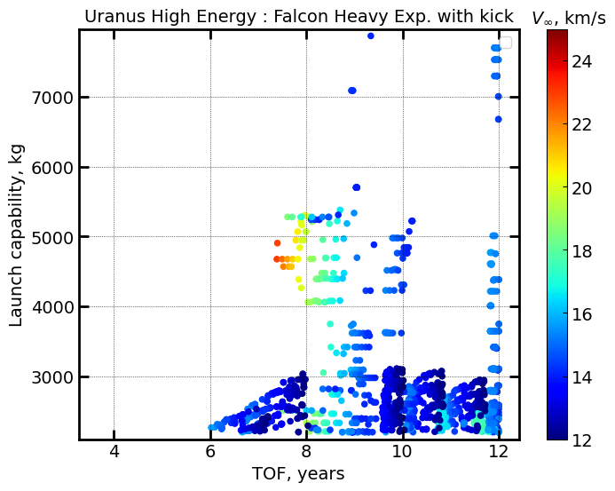
It appears that there is small set of trajectories (indicated by yellow and red markers) which satisfy the following constraints:
Launch capability >= 5000 kg with Falcon Heavy Expendable. (corresponding to \(C_3\) <= 55)
TOF <= 8 years.
Arrival \(V_{\infty}\) >= 20 km/s, and \(V_{\infty}\) <= 24 km/s.
We perform a query on the interplanetary trajectory dataset to filter these trajectories.
[7]:
df = interplanetary1.df
df[(df["TOF"]<=8) & (df["Avinf"]>=20) & (df["Avinf"]<=24) & (df["LC3"]<=55)]
[7]:
| Bodies | Times | Lcdate | Arrival Date | LC3 | TOF | DSMdv | DSM Mass | ArrivalVinf_Vector | Avinf | Adec | Unnamed: 11 | Paths | Unnamed: 13 | Unnamed: 14 | |
|---|---|---|---|---|---|---|---|---|---|---|---|---|---|---|---|
| 11717 | [399 399 599 799] | 2031-07-18 2034-05-16 2035-09-09 2039-06-07 | 2031-07-18 | 2039-06-07 | 52.266 | 7.886090 | 1.04 | 864.379658 | [-9.511251449584961 17.8606014251709 0.2777369... | 20.237 | -48.836271 | NaN | NaN | NaN | NaN |
| 11740 | [399 399 599 799] | 2031-07-22 2034-05-16 2035-09-04 2039-05-18 | 2031-07-22 | 2039-05-18 | 53.866 | 7.820462 | 1.04 | 864.379658 | [-9.630807876586914 18.130252838134766 0.28104... | 20.531 | -48.894486 | NaN | NaN | NaN | NaN |
| 11745 | [399 399 599 799] | 2031-07-22 2034-05-24 2035-09-14 2039-06-17 | 2031-07-22 | 2039-06-17 | 52.823 | 7.902598 | 0.84 | 675.544505 | [-9.463287353515625 17.745807647705078 0.27622... | 20.113 | -48.803860 | NaN | NaN | NaN | NaN |
We see that these trajectories belong to a group of EEJU trajectories launching between July and August 2031. For preliminary analysis, we arbitrarily choose trajectory #11740 as the initial baseline. We will now use the AMAT.arrival module to compute the arrival \(V_{\infty}\) and arrival declination for this trajectory.
[8]:
from astropy.time import Time
from AMAT.arrival import Arrival

arrival = Arrival()
arrival.set_vinf_vec_from_lambert_arc('JUPITER',
                                      'URANUS',
                                      Time("2035-09-04 00:00:00", scale='tdb'),
                                      Time("2039-05-18 00:00:00", scale='tdb'))
[9]:
arrival.v_inf_vec
[9]:
array([-9.62521831, 16.51192666, 7.46493598])
[10]:
arrival.declination
[10]:
-48.89326200262988
We now compute an approach trajectory that minimizes the inclination of the initial capture orbit with respect to Uranus’ equatorial plane. Note that the entry conditions (except the EFPA) is required to compute the aerocapture ebtry corridor, and hence this must be done iteratively. We arbitrarily choose an initial periapsis radius = 400 km which results in a planet-relative EFPA of -11.1 deg.
[11]:
import numpy as np
from AMAT.approach import Approach
[12]:
approach1 = Approach("URANUS", v_inf_vec_icrf_kms=arrival.v_inf_vec,
                            rp=(25559+400)*1e3, psi=3*np.pi/2,
                            is_entrySystem=True, h_EI=1000e3)

print("Entry altitude, km: "+ str(approach1.h_EI/1e3))
print("Entry longitude BI, deg: "+ str(round(approach1.longitude_entry_bi*180/np.pi, 2)))
print("Entry latitude BI, deg: "+ str(round(approach1.latitude_entry_bi*180/np.pi, 2)))
print("Atm. relative entry speed, km/s: "+str(round(approach1.v_entry_atm_mag/1e3, 4)))
print("Atm. relative heading angle, deg: "+str(round(approach1.heading_entry_atm*180/np.pi, 4)))
print("Atm. relative EFPA, deg: "+str(round(approach1.gamma_entry_atm*180/np.pi, 4)))
Entry altitude, km: 1000.0
Entry longitude BI, deg: -80.95
Entry latitude BI, deg: 25.22
Atm. relative entry speed, km/s: 27.5946
Atm. relative heading angle, deg: 132.066
Atm. relative EFPA, deg: -11.1875
Run the file example-72-uranus-approach.py for a visualization of the Uranus approach trajectory.
[13]:
Image(filename="../plots/example-72-uranus-approach.png", width=700)
[13]:
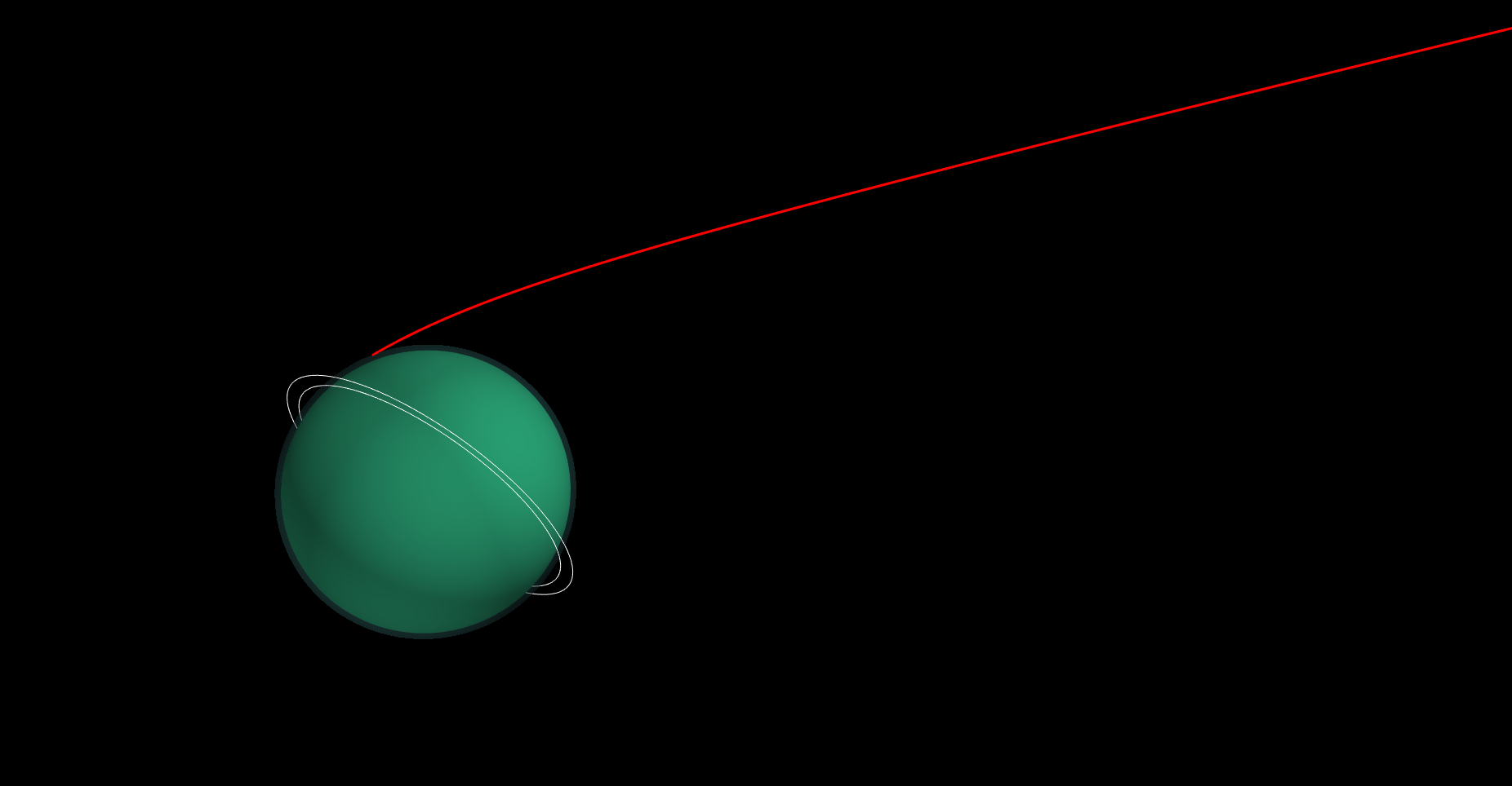
Using the above entry conditions at Uranus atmospheric interface, we use AMAT.vehicle module to compute the aerocapture entry corridor for a vehicle with L/D = 0.36 and a nominal mean atmospheric profile for Uranus.
[14]:
# setup the Planet object
from AMAT.planet import Planet
planet=Planet("URANUS")
planet.h_skip = 1000e3
planet.loadAtmosphereModel('../atmdata/Uranus/uranus-gram-avg.dat', 0 , 1 ,2, 3, heightInKmFlag=True)
planet.h_low = 120e3
planet.h_trap= 100e3
[15]:
# Setup the vehicle object : assume m=3000 kg, beta=200 kg/m2
from AMAT.vehicle import Vehicle
vehicle=Vehicle('Titania', 3000.0, 200 , 0.36, np.pi*4.5**2.0, 0.0, 1.125, planet)
vehicle.setInitialState(1000.0,-80.95,25.22,27.5946,132.066,-11.0 ,0.0,0.0)
vehicle.setSolverParams(1E-6)
[16]:
# Compute the corridor bounds and TCW
overShootLimit, exitflag_os  = vehicle.findOverShootLimit2(2400.0,0.1,-25,-4.0,1E-10,500e3)
underShootLimit, exitflag_us  = vehicle.findUnderShootLimit2(2400.0,0.1,-25 ,-4.0,1E-10,500e3)
[17]:
# print the overshoot and undershoot limits we just computed.
print("Overshoot  limit : "+str('{:.4f}'.format(overShootLimit))+ " deg")
print("Undershoot limit : "+str('{:.4f}'.format(underShootLimit))+ " deg")
print("TCW: "+ str('{:.4f}'.format(overShootLimit-underShootLimit))+ " deg")
Overshoot  limit : -11.7077 deg
Undershoot limit : -13.4105 deg
TCW: 1.7029 deg
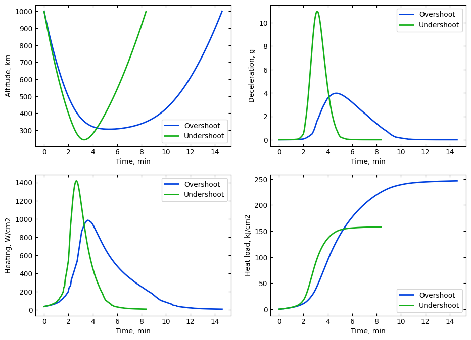
[18]:
# propogate the overshoot and undershoot trajectories
vehicle.setInitialState(1000.0,-80.95,25.22,27.5946,132.066,overShootLimit ,0.0,0.0)
vehicle.propogateEntry (2400.0,0.1,180.0)

# Extract and save variables to plot
t_min_os         = vehicle.t_minc
h_km_os          = vehicle.h_kmc
acc_net_g_os     = vehicle.acc_net_g
q_stag_con_os    = vehicle.q_stag_con
q_stag_rad_os    = vehicle.q_stag_rad
heatload_os      = vehicle.heatload

vehicle.setInitialState(1000.0,-80.95,25.22,27.5946,132.066,underShootLimit ,0.0,0.0)
vehicle.propogateEntry (2400.0,0.1,0.0)

# Extract and save variable to plot
t_min_us         = vehicle.t_minc
h_km_us          = vehicle.h_kmc
acc_net_g_us     = vehicle.acc_net_g
q_stag_con_us    = vehicle.q_stag_con
q_stag_rad_us    = vehicle.q_stag_rad
heatload_us      = vehicle.heatload
[19]:
# plot overshoot and undershoot trajectories
fig = plt.figure()
fig.set_size_inches([11 , 8])
params = {'mathtext.default': 'regular' }
plt.rcParams.update(params)

plt.subplot(2, 2, 1)
plt.plot(t_min_os , h_km_os, linestyle='solid' , color='xkcd:blue',linewidth=2.0,  label='Overshoot')
plt.plot(t_min_us , h_km_us, linestyle='solid' , color='xkcd:green',linewidth=2.0,  label='Undershoot')
plt.xlabel('Time, min',fontsize=10)
plt.ylabel("Altitude, km",fontsize=10)
ax = plt.gca()
ax.tick_params(direction='in')
ax.yaxis.set_ticks_position('both')
ax.xaxis.set_ticks_position('both')
plt.tick_params(direction='in')
plt.tick_params(axis='x',labelsize=10)
plt.tick_params(axis='y',labelsize=10)
plt.legend(loc='lower right', fontsize=10)


plt.subplot(2, 2, 2)
plt.plot(t_min_os , acc_net_g_os , linestyle='solid' , color='xkcd:blue',linewidth=2.0,  label='Overshoot')
plt.plot(t_min_us , acc_net_g_us, linestyle='solid' , color='xkcd:green',linewidth=2.0,  label='Undershoot')
plt.xlabel('Time, min',fontsize=10)
plt.ylabel("Deceleration, g",fontsize=10)
ax = plt.gca()
ax.tick_params(direction='in')
ax.yaxis.set_ticks_position('both')
ax.xaxis.set_ticks_position('both')
plt.tick_params(direction='in')
plt.tick_params(axis='x',labelsize=10)
plt.tick_params(axis='y',labelsize=10)
plt.legend(loc='upper right', fontsize=10)

plt.subplot(2, 2, 3)
plt.plot(t_min_os , q_stag_con_os+q_stag_rad_os, linestyle='solid' , color='xkcd:blue',linewidth=2.0,  label='Overshoot')
plt.plot(t_min_us , q_stag_con_us+q_stag_rad_us, linestyle='solid' , color='xkcd:green',linewidth=2.0,  label='Undershoot')
plt.xlabel('Time, min',fontsize=10)
plt.ylabel("Heating, W/cm2",fontsize=10)
ax = plt.gca()
ax.tick_params(direction='in')
ax.yaxis.set_ticks_position('both')
ax.xaxis.set_ticks_position('both')
plt.tick_params(direction='in')
plt.tick_params(axis='x',labelsize=10)
plt.tick_params(axis='y',labelsize=10)
plt.legend(loc='upper right', fontsize=10)

plt.subplot(2, 2, 4)
plt.plot(t_min_os , heatload_os/1e3 , linestyle='solid' , color='xkcd:blue',linewidth=2.0,  label='Overshoot')
plt.plot(t_min_us , heatload_us/1e3, linestyle='solid' , color='xkcd:green',linewidth=2.0,  label='Undershoot')
plt.xlabel('Time, min',fontsize=10)
plt.ylabel("Heat load, kJ/cm2",fontsize=10)
ax = plt.gca()
ax.tick_params(direction='in')
ax.yaxis.set_ticks_position('both')
ax.xaxis.set_ticks_position('both')
plt.tick_params(direction='in')
plt.tick_params(axis='x',labelsize=10)
plt.tick_params(axis='y',labelsize=10)
plt.legend(loc='lower right', fontsize=10)


plt.show()