Example - 08 - Venus Aerocapture: Part 4

In this example, you will learn to create a drag modulation aerocapture feasibility chart for Venus.

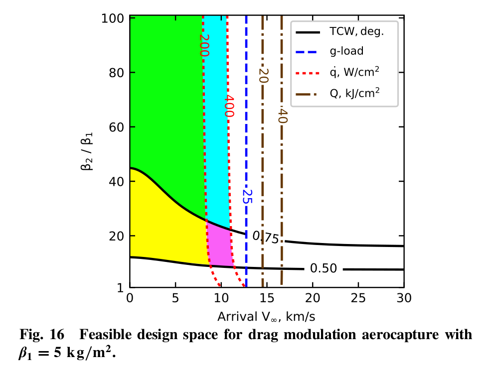
For reference, we will re-create another figure from the paper “Girija, Lu, and Saikia, Feasibility and Mass-Benefit Analysis of Aerocapture for Missions to Venus, Journal of Spacecraft and Rockets, Vol. 57, No. 1” DOI: 10.2514/1.A34529

[1]:

from IPython.display import Image
Image(filename='../plots/girijaYe2020c-reference.png', width=600)

[1]:

../_images/examples_example-08-venus-aerocapture-4_2_0.png

[2]:

from AMAT.planet import Planet
from AMAT.vehicle import Vehicle

import numpy as np
from scipy import interpolate

import matplotlib.pyplot as plt
from matplotlib import rcParams
from matplotlib.patches import Polygon
import os

[3]:

# Create a planet object
planet=Planet("VENUS")
planet.h_skip = 150000.0

# Load an nominal atmospheric profile with height, temp, pressure, density data
planet.loadAtmosphereModel('../atmdata/Venus/venus-gram-avg.dat', 0 , 1 ,2, 3)

vinf_kms_array  = np.linspace( 0.0,   30.0,   11)
betaRatio_array = np.linspace( 1.0,   101.0 , 11)

#vinf_kms_array  = np.linspace( 0.0,   30.0,   2)
#betaRatio_array = np.linspace( 1.0,   101.0 , 2)

[4]:

beta1 = 5.0

os.makedirs('../data/girijaYe2019c')
runID = 'DMBC5RAP400EI150'

[5]:

v0_kms_array    = np.zeros(len(vinf_kms_array))
v0_kms_array[:] = np.sqrt(1.0*(vinf_kms_array[:]*1E3)**2.0 + 2*np.ones(len(vinf_kms_array))*planet.GM/(planet.RP+150.0*1.0E3))/1.0E3

overShootLimit_array  = np.zeros((len(v0_kms_array),len(betaRatio_array)))
underShootLimit_array = np.zeros((len(v0_kms_array),len(betaRatio_array)))
exitflag_os_array     = np.zeros((len(v0_kms_array),len(betaRatio_array)))
exitflag_us_array     = np.zeros((len(v0_kms_array),len(betaRatio_array)))
TCW_array             = np.zeros((len(v0_kms_array),len(betaRatio_array)))

[6]:

for i in range(0,len(v0_kms_array)):
    for j in range(0,len(betaRatio_array)):
        vehicle=Vehicle('DMVehicle', 1500.0, beta1, 0.0, 3.1416, 0.0, 0.10, planet)
        vehicle.setInitialState(150.0,0.0,0.0,v0_kms_array[i],0.0,-4.5,0.0,0.0)
        vehicle.setSolverParams(1E-6)
        vehicle.setDragModulationVehicleParams(beta1,betaRatio_array[j])

        underShootLimit_array[i,j], exitflag_us_array[i,j] = vehicle.findUnderShootLimitD(2400.0, 0.1, -80.0,-4.0,1E-10,400.0)
        overShootLimit_array[i,j] , exitflag_os_array[i,j] = vehicle.findOverShootLimitD (2400.0, 0.1, -80.0,-4.0,1E-10,400.0)

        TCW_array[i,j]    = overShootLimit_array[i,j] - underShootLimit_array[i,j]

        print('VINF: '+str(vinf_kms_array[i])+' km/s, BETA RATIO: '+str(betaRatio_array[j])+' TCW: '+str(TCW_array[i,j])+' deg.')

np.savetxt('../data/girijaYe2019c/'+runID+'vinf_kms_array.txt',vinf_kms_array)
np.savetxt('../data/girijaYe2019c/'+runID+'v0_kms_array.txt',v0_kms_array)
np.savetxt('../data/girijaYe2019c/'+runID+'betaRatio_array.txt',betaRatio_array)
np.savetxt('../data/girijaYe2019c/'+runID+'overShootLimit_array.txt',overShootLimit_array)
np.savetxt('../data/girijaYe2019c/'+runID+'exitflag_os_array.txt',exitflag_os_array)
np.savetxt('../data/girijaYe2019c/'+runID+'underShootLimit_array.txt',underShootLimit_array)
np.savetxt('../data/girijaYe2019c/'+runID+'exitflag_us_array.txt',exitflag_us_array)
np.savetxt('../data/girijaYe2019c/'+runID+'TCW_array.txt',TCW_array)

VINF: 0.0 km/s, BETA RATIO: 1.0 TCW: 0.0 deg.
VINF: 0.0 km/s, BETA RATIO: 101.0 TCW: 0.8981981236029242 deg.
VINF: 30.0 km/s, BETA RATIO: 1.0 TCW: 0.0 deg.
VINF: 30.0 km/s, BETA RATIO: 101.0 TCW: 1.192248803385155 deg.

[8]:

acc_net_g_max_array       = np.zeros((len(v0_kms_array),len(betaRatio_array)))
stag_pres_atm_max_array   = np.zeros((len(v0_kms_array),len(betaRatio_array)))
q_stag_total_max_array    = np.zeros((len(v0_kms_array),len(betaRatio_array)))
heatload_max_array        = np.zeros((len(v0_kms_array),len(betaRatio_array)))


for i in range(0,len(v0_kms_array)):
    for j in range(0,len(betaRatio_array)):
        vehicle=Vehicle('DMVehicle', 1500.0, beta1, 0.0, 3.1416, 0.0, 0.10, planet)
        vehicle.setInitialState(150.0,0.0,0.0,v0_kms_array[i],0.0,overShootLimit_array[i,j],0.0,0.0)
        vehicle.setSolverParams(1E-6)

        vehicle.propogateEntry (2400.0, 0.1, 0.0)

        # Extract and save variables to plot
        t_min_os         = vehicle.t_minc
        h_km_os          = vehicle.h_kmc
        acc_net_g_os     = vehicle.acc_net_g
        q_stag_con_os    = vehicle.q_stag_con
        q_stag_rad_os    = vehicle.q_stag_rad
        rc_os            = vehicle.rc
        vc_os            = vehicle.vc
        stag_pres_atm_os = vehicle.computeStagPres(rc_os,vc_os)/(1.01325E5)
        heatload_os      = vehicle.heatload


        vehicle=Vehicle('DMVehicle', 1500.0, beta1*betaRatio_array[j], 0.0, 3.1416, 0.0, 0.10, planet)
        vehicle.setInitialState(150.0,0.0,0.0,v0_kms_array[i],0.0,underShootLimit_array[i,j],0.0,0.0)
        vehicle.setSolverParams( 1E-6)

        vehicle.propogateEntry (2400.0, 0.1, 0.0)

        # Extract and save variable to plot
        t_min_us         = vehicle.t_minc
        h_km_us          = vehicle.h_kmc
        acc_net_g_us     = vehicle.acc_net_g
        q_stag_con_us    = vehicle.q_stag_con
        q_stag_rad_us    = vehicle.q_stag_rad
        rc_us            = vehicle.rc
        vc_us            = vehicle.vc
        stag_pres_atm_us = vehicle.computeStagPres(rc_us,vc_us)/(1.01325E5)
        heatload_us      = vehicle.heatload

        q_stag_total_os  = q_stag_con_os + q_stag_rad_os
        q_stag_total_us  = q_stag_con_us + q_stag_rad_us

        acc_net_g_max_array[i,j]      = max(max(acc_net_g_os),max(acc_net_g_us))
        stag_pres_atm_max_array[i,j]  = max(max(stag_pres_atm_os),max(stag_pres_atm_os))
        q_stag_total_max_array[i,j]   = max(max(q_stag_total_os),max(q_stag_total_us))
        heatload_max_array[i,j]       = max(max(heatload_os),max(heatload_us))

        print("V_infty: "+str(vinf_kms_array[i])+" km/s"+", BR: "+str(betaRatio_array[j])+" G_MAX: "+str(acc_net_g_max_array[i,j])+" QDOT_MAX: "+str(q_stag_total_max_array[i,j])+" J_MAX: "+str(heatload_max_array[i,j])+" STAG. PRES: "+str(stag_pres_atm_max_array[i,j]))

np.savetxt('../data/girijaYe2019c/'+runID+'acc_net_g_max_array.txt',acc_net_g_max_array)
np.savetxt('../data/girijaYe2019c/'+runID+'stag_pres_atm_max_array.txt',stag_pres_atm_max_array)
np.savetxt('../data/girijaYe2019c/'+runID+'q_stag_total_max_array.txt',q_stag_total_max_array)
np.savetxt('../data/girijaYe2019c/'+runID+'heatload_max_array.txt',heatload_max_array)

V_infty: 0.0 km/s, BR: 1.0 G_MAX: 4.2619678756684065 QDOT_MAX: 107.04783114721339 J_MAX: 9963.95886102549 STAG. PRES: 0.00206384918146089
V_infty: 0.0 km/s, BR: 101.0 G_MAX: 4.2619678756684065 QDOT_MAX: 1069.8045659113661 J_MAX: 105153.41622997135 STAG. PRES: 0.00206384918146089
V_infty: 30.0 km/s, BR: 1.0 G_MAX: 143.43437041606074 QDOT_MAX: 763604.549664235 J_MAX: 4964898.795992032 STAG. PRES: 0.06941820444237855
V_infty: 30.0 km/s, BR: 101.0 G_MAX: 143.43437041606074 QDOT_MAX: 182872814.4356986 J_MAX: 1231040818.2242763 STAG. PRES: 0.06941820444237855

[9]:

x = np.loadtxt('../data/girijaYe2019c/'+runID+'vinf_kms_array.txt')
y = np.loadtxt('../data/girijaYe2019c/'+runID+'betaRatio_array.txt')

Z1 = np.loadtxt('../data/girijaYe2019c/'+runID+'TCW_array.txt')
G1 = np.loadtxt('../data/girijaYe2019c/'+runID+'acc_net_g_max_array.txt')
Q1 = np.loadtxt('../data/girijaYe2019c/'+runID+'q_stag_total_max_array.txt')
H1 = np.loadtxt('../data/girijaYe2019c/'+runID+'heatload_max_array.txt')
S1 = np.loadtxt('../data/girijaYe2019c/'+runID+'stag_pres_atm_max_array.txt')


f1 = interpolate.interp2d(x, y, np.transpose(Z1), kind='cubic')
g1 = interpolate.interp2d(x, y, np.transpose(G1), kind='cubic')
q1 = interpolate.interp2d(x, y, np.transpose(Q1), kind='cubic')
h1 = interpolate.interp2d(x, y, np.transpose(H1), kind='cubic')
s1 = interpolate.interp2d(x, y, np.transpose(S1), kind='cubic')


x_new =  np.linspace( 0.0,   30,  110)
y_new =  np.linspace( 0.0,   101 ,110)

z1_new =  np.zeros((len(x_new),len(y_new)))
g1_new =  np.zeros((len(x_new),len(y_new)))
q1_new =  np.zeros((len(x_new),len(y_new)))
h1_new =  np.zeros((len(x_new),len(y_new)))
s1_new =  np.zeros((len(x_new),len(y_new)))

for i in range(0,len(x_new)):
    for j in range(0,len(y_new)):

        z1_new[i,j] = f1(x_new[i],y_new[j])
        g1_new[i,j] = g1(x_new[i],y_new[j])
        q1_new[i,j] = q1(x_new[i],y_new[j])
        h1_new[i,j] = h1(x_new[i],y_new[j])
        s1_new[i,j] = s1(x_new[i],y_new[j])


Z1 = z1_new
G1 = g1_new
Q1 = q1_new
S1 = s1_new
H1 = h1_new/1000.0

X, Y = np.meshgrid(x_new, y_new)

Zlevels = np.array([0.5,0.75])
Glevels = np.array([25.0])
Qlevels = np.array([200.0, 400.0])
Hlevels = np.array([20.0,40.0])

fig = plt.figure()
fig.set_size_inches([3.25,3.25])
plt.ion()
plt.rc('font',family='Times New Roman')
params = {'mathtext.default': 'regular' }
plt.rcParams.update(params)

ZCS1 = plt.contour(X, Y, np.transpose(Z1), levels=Zlevels, colors='black')
plt.clabel(ZCS1, inline=1, fontsize=10, colors='black',fmt='%.2f',inline_spacing=1)
ZCS1.collections[0].set_linewidths(1.50)
ZCS1.collections[1].set_linewidths(1.50)
ZCS1.collections[0].set_label(r'$TCW, deg.$')

GCS1 = plt.contour(X, Y, np.transpose(G1), levels=Glevels, colors='blue',linestyles='dashed')
Glabels=plt.clabel(GCS1, inline=1, fontsize=10, colors='blue',fmt='%d',inline_spacing=0)
GCS1.collections[0].set_linewidths(1.50)

GCS1.collections[0].set_label(r'$g$'+r'-load')

QCS1 = plt.contour(X, Y, np.transpose(Q1), levels=Qlevels, colors='red',linestyles='dotted',zorder=11)
plt.clabel(QCS1, inline=1, fontsize=10, colors='red',fmt='%d',inline_spacing=0)
QCS1.collections[0].set_linewidths(1.50)
QCS1.collections[1].set_linewidths(1.50)
QCS1.collections[0].set_label(r'$\dot{q}$'+', '+r'$W/cm^2$')


HCS1 = plt.contour(X, Y, np.transpose(H1), levels=Hlevels, colors='xkcd:brown',linestyles='dashdot')
Hlabels=plt.clabel(HCS1, inline=1, fontsize=10, colors='xkcd:brown',fmt='%d',inline_spacing=0)
HCS1.collections[0].set_linewidths(1.75)
HCS1.collections[1].set_linewidths(1.75)
HCS1.collections[0].set_label(r'$Q$'+', '+r'$kJ/cm^2$')

for l in Hlabels:
    l.set_rotation(-90)
for l in Glabels:
    l.set_rotation(-90)


#SCS1 = plt.contour(X, Y, transpose(S1), levels=Slevels, colors='cyan')
#plt.clabel(SCS1, inline=1, fontsize=10, colors='xkcd:neon green',fmt='%.1f',inline_spacing=1)
#SCS1.collections[0].set_linewidths(1.75)
#SCS1.collections[0].set_label(r'$Peak$'+r' '+r'$stag. pressure,atm$')

plt.xlabel("Arrival "+r'$V_\infty$'+r', km/s' ,fontsize=10)
plt.ylabel(r'$\beta_2$'+' / '+r'$ \beta_1 $' ,fontsize=10)
plt.xticks(fontsize=10)
plt.yticks(np.array([ 1, 20, 40, 60, 80, 100]),fontsize=10)
ax = plt.gca()
ax.tick_params(direction='in')
ax.yaxis.set_ticks_position('both')
ax.xaxis.set_ticks_position('both')
plt.legend(loc='upper right', fontsize=8)


dat0 = ZCS1.allsegs[1][0]
x1,y1=dat0[:,0],dat0[:,1]
F1 = interpolate.interp1d(x1, y1, kind='linear',fill_value='extrapolate', bounds_error=False)

dat1 = QCS1.allsegs[0][0]
x2,y2=dat1[:,0],dat1[:,1]
F2 = interpolate.interp1d(x2, y2, kind='linear',fill_value='extrapolate', bounds_error=False)

dat0a = ZCS1.allsegs[0][0]
x1a,y1a=dat0a[:,0],dat0a[:,1]
F1a = interpolate.interp1d(x1a, y1a, kind='linear',fill_value='extrapolate', bounds_error=False)


x3 = np.linspace(0,30,301)
y3 = F1(x3)
y4 = F2(x3)
y4a =F1a(x3)

y8 = np.minimum(y3,y4)


plt.fill_between(x3, y3, y4, where=y3<=y4, color='xkcd:neon green')
plt.fill_between(x3, y4a, y8, where=y4a<=y8, color='xkcd:bright yellow')

plt.xlim([0.0,30.0])
plt.ylim([1.0,100])


plt.savefig('../plots/girijaYe2019c-fig16.png',bbox_inches='tight')
plt.savefig('../plots/girijaYe2019c-fig16.pdf', dpi=300,bbox_inches='tight')
plt.savefig('../plots/girijaYe2019c-fig16.eps', dpi=300,bbox_inches='tight')

plt.show()

/home/athul/anaconda3/lib/python3.7/site-packages/scipy/interpolate/interpolate.py:609: RuntimeWarning: divide by zero encountered in true_divide
  slope = (y_hi - y_lo) / (x_hi - x_lo)[:, None]
The PostScript backend does not support transparency; partially transparent artists will be rendered opaque.
The PostScript backend does not support transparency; partially transparent artists will be rendered opaque.
The PostScript backend does not support transparency; partially transparent artists will be rendered opaque.
The PostScript backend does not support transparency; partially transparent artists will be rendered opaque.

../_images/examples_example-08-venus-aerocapture-4_9_1.png

[10]:

from IPython.display import Image
Image(filename='../plots/girijaYe2020c-higher-res.png', width=600)

[10]:

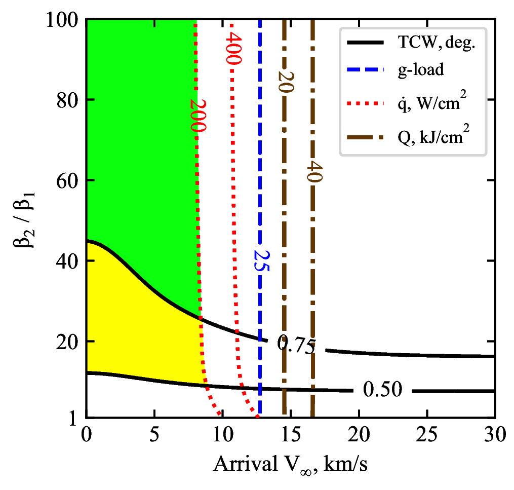
../_images/examples_example-08-venus-aerocapture-4_10_0.png

The plots are now saved in plots/girijaYe2019c.

Congratulations! You could now create the results for referenced journal article in less than a day. It took nearly a year for the authors to put everything together to create these results!