Example - 11 - Neptune Aerocapture - Part 2a: Monte Carlo Simulations
In this example, we will use AMAT to perform Monte Carlo simulations to assess aerocapture vehicle performance.
We reproduce the example Monte Carlo results from “Girija, Saikia, Longuski et al. Feasibility and Performance Analysis of Neptune Aerocapture Using Heritage Blunt-Body Aeroshells, Journal of Spacecraft and Rockets, June, 2020, In press. DOI: 10.2514/1.A34719. Refer Section VIII A: Results for prograde entry with maximum range of FMINMAX.
[1]:
from AMAT.planet import Planet
from AMAT.vehicle import Vehicle

import numpy as np
from scipy import interpolate
import pandas as pd

import matplotlib.pyplot as plt
from matplotlib import rcParams
from matplotlib.patches import Polygon
[2]:
# Create a planet object
planet=Planet("NEPTUNE")

# Load an nominal atmospheric profile with height, temp, pressure, density data
planet.loadAtmosphereModel('../atmdata/Neptune/neptune-gram-avg.dat', 0 , 7 , 6 , 5 , \
                            heightInKmFlag=True)

# Create a vehicle object
vehicle=Vehicle('Trident', 1000.0, 200.0, 0.40, 3.1416, 0.0, 1.00, planet)

# Set vehicle conditions at entry interface
# The EFPA selection process is described in Sec. VII in the reference article.
vehicle.setInitialState(1000.0, 0.0, 0.0, 28.00, 0.0,-13.85, 0.0, 0.0)
vehicle.setSolverParams(1E-6)
[3]:
# Set the guidance parameters described in the paper.
# See the function description for parameter details.

# Set max roll rate constraint to 30 deg/s
vehicle.setMaxRollRate(30.0)

# Set Ghdot = 75
# Set Gq = 3.0
# Set v_switch_kms = 18.9
# Set low_Alt_km = 120
# Set numPoints_lowAlt = 101
# Set hdot_threshold = -500 m/s
vehicle.setEquilibriumGlideParams(75.0, 3.0, 18.9, 120.0, 101, -500.0)

# Set target orbit parameters
# periapsis = 4000.0 km
# apoapsis = 400,000 km
# apoapsis tolerance = 10 km
vehicle.setTargetOrbitParams(4000.0, 400.0E3, 10.0E3)
[4]:
# Set path to atmfiles with randomly perturbed atmosphere files.

atmfiles = ['../atmdata/Neptune/FMINMAX-10L.txt',
            '../atmdata/Neptune/FMINMAX-08L.txt',
            '../atmdata/Neptune/FMINMAX-06L.txt',
            '../atmdata/Neptune/FMINMAX-04L.txt',
            '../atmdata/Neptune/FMINMAX-02L.txt',
            '../atmdata/Neptune/FMINMAX+00L.txt',
            '../atmdata/Neptune/FMINMAX+02L.txt',
            '../atmdata/Neptune/FMINMAX+04L.txt',
            '../atmdata/Neptune/FMINMAX+06L.txt',
            '../atmdata/Neptune/FMINMAX+08L.txt',
            '../atmdata/Neptune/FMINMAX+10L.txt']
[5]:
# Set up Monte Carlo simulation parameters

# See function description for details.

# NPOS = 1086
# NMONTE = 200

vehicle.setupMonteCarloSimulation(1086, 200, atmfiles, 0, 1, 2, 3, 4, True, \
                                 -13.85, 0.11, 0.40, 0.013, 0.5, 0.1, 2400.0)
[6]:
# Run the Monte Carlo simulation.

# N = 10 shown here, run for a few thousand to be realistic. This will take several hours.

vehicle.runMonteCarlo(10, '../data/girijaSaikia2020a/MCB1')
BATCH :../data/girijaSaikia2020a/MCBX, RUN #: 1, PROF: ../atmdata/Neptune/FMINMAX-04L.txt, SAMPLE #: 22, EFPA: -13.97, SIGMA: -1.04, LD: 0.41, APO : 379646.10
BATCH :../data/girijaSaikia2020a/MCBX, RUN #: 2, PROF: ../atmdata/Neptune/FMINMAX+10L.txt, SAMPLE #: 194, EFPA: -13.86, SIGMA: 1.66, LD: 0.39, APO : 397722.98
BATCH :../data/girijaSaikia2020a/MCBX, RUN #: 3, PROF: ../atmdata/Neptune/FMINMAX+04L.txt, SAMPLE #: 188, EFPA: -13.89, SIGMA: -0.71, LD: 0.39, APO : 367641.10
BATCH :../data/girijaSaikia2020a/MCBX, RUN #: 4, PROF: ../atmdata/Neptune/FMINMAX+10L.txt, SAMPLE #: 125, EFPA: -13.79, SIGMA: -1.81, LD: 0.41, APO : 360589.69
BATCH :../data/girijaSaikia2020a/MCBX, RUN #: 5, PROF: ../atmdata/Neptune/FMINMAX-02L.txt, SAMPLE #: 172, EFPA: -13.83, SIGMA: 1.24, LD: 0.40, APO : 383384.65
BATCH :../data/girijaSaikia2020a/MCBX, RUN #: 6, PROF: ../atmdata/Neptune/FMINMAX+02L.txt, SAMPLE #: 29, EFPA: -13.77, SIGMA: -0.44, LD: 0.39, APO : 372647.16
BATCH :../data/girijaSaikia2020a/MCBX, RUN #: 7, PROF: ../atmdata/Neptune/FMINMAX-04L.txt, SAMPLE #: 63, EFPA: -13.71, SIGMA: 0.76, LD: 0.39, APO : 376441.97
BATCH :../data/girijaSaikia2020a/MCBX, RUN #: 8, PROF: ../atmdata/Neptune/FMINMAX+00L.txt, SAMPLE #: 162, EFPA: -13.67, SIGMA: -2.19, LD: 0.41, APO : 380977.85
BATCH :../data/girijaSaikia2020a/MCBX, RUN #: 9, PROF: ../atmdata/Neptune/FMINMAX+06L.txt, SAMPLE #: 60, EFPA: -13.73, SIGMA: 0.86, LD: 0.40, APO : 382393.74
BATCH :../data/girijaSaikia2020a/MCBX, RUN #: 10, PROF: ../atmdata/Neptune/FMINMAX+00L.txt, SAMPLE #: 161, EFPA: -13.77, SIGMA: 0.79, LD: 0.40, APO : 368610.27
[7]:
# Post process Monte Carlo simulation data.


peri  = np.loadtxt('../data/girijaSaikia2020a/MCB1/terminal_periapsis_arr.txt')
apoa  = np.loadtxt('../data/girijaSaikia2020a/MCB1/terminal_apoapsis_arr.txt')

peri_dv  = np.loadtxt('../data/girijaSaikia2020a/MCB1/periapsis_raise_DV_arr.txt')

del_index1 = np.where(apoa < 0)
del_index2 = np.where(apoa>800.0E3)

del_index = np.concatenate((del_index1, del_index2), axis=1)

print('Simulation statistics')
print('----------------------------------------------')
print("No. of cases escaped :"+str(len(del_index1[0])))
print("No. of cases with apo. alt > 800.0E3 km :"+str(len(del_index2[0])))
Simulation statistics
----------------------------------------------
No. of cases escaped :3
No. of cases with apo. alt > 800.0E3 km :0
[8]:
# Remove escaped cases before plotting
peri_new = np.delete(peri, del_index)
apoa_new = np.delete(apoa, del_index)
peri_dv_new  = np.delete(peri_dv, del_index)
[9]:
# Create apoapsis dispersion plot.

fig = plt.figure()
fig.set_size_inches([3.25,3.25])
plt.rc('font',family='Times New Roman')
params = {'mathtext.default': 'regular' }
plt.rcParams.update(params)

plt.plot(peri_new, apoa_new/1000.0, 'bo', markersize=3)

plt.xlabel('Periapsis altitude, km',fontsize=10)
plt.ylabel('Apoapsis altitude x '+r'$10^3$'+', km', fontsize=10)

plt.axhline(y=350.0, linewidth=1, color='k', linestyle='dotted')
plt.axhline(y=450.0, linewidth=1, color='k', linestyle='dotted')

ax=plt.gca()
ax.tick_params(direction='in')
ax.yaxis.set_ticks_position('both')
ax.xaxis.set_ticks_position('both')
ax.tick_params(axis='x',labelsize=10)
ax.tick_params(axis='y',labelsize=10)

plt.savefig('../plots/girijaSaikia2020a-fig-15-N100.png',bbox_inches='tight')
plt.savefig('../plots/girijaSaikia2020a-fig-15-N100.pdf', dpi=300,bbox_inches='tight')
plt.savefig('../plots/girijaSaikia2020a-fig-15-N100.eps', dpi=300,bbox_inches='tight')
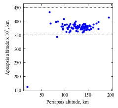
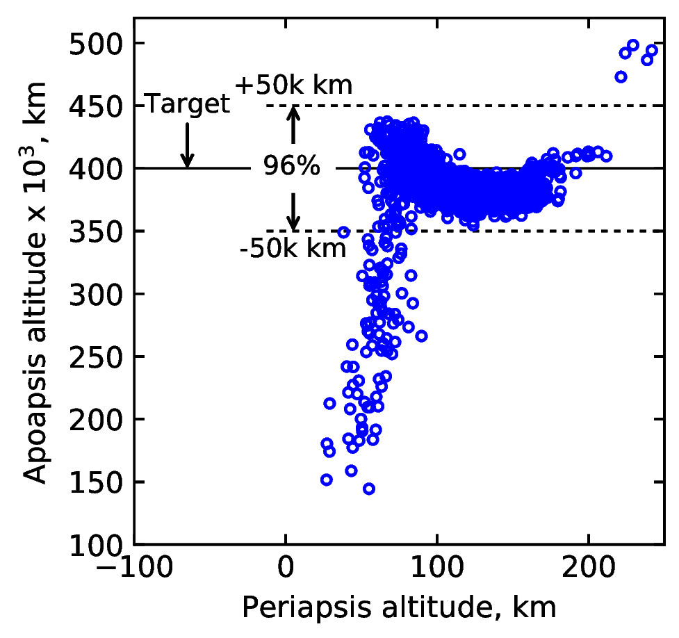
This plot only has 100 trajectories. Below is a similar plot with 5000 trajectories
[15]:
from IPython.display import Image
Image(filename='../plots/prograde-higher-res.png', width=600)
[15]:
[13]:
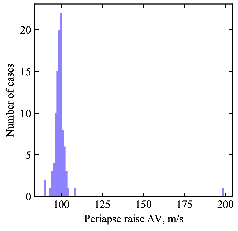
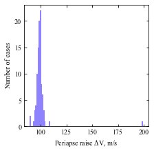
# Create histogram of periapse raise manuever DV

fig = plt.figure()
fig.set_size_inches([3.25,3.25])
plt.rc('font',family='Times New Roman')
params = {'mathtext.default': 'regular' }
plt.rcParams.update(params)

plt.hist(peri_dv_new, bins=100, color='xkcd:periwinkle')
plt.xlabel('Periapse raise '+r'$\Delta V$'+', m/s', fontsize=10)
plt.ylabel('Number of cases', fontsize=10)
ax=plt.gca()
ax.tick_params(direction='in')
ax.yaxis.set_ticks_position('both')
ax.xaxis.set_ticks_position('both')
ax.tick_params(axis='x',labelsize=10)
ax.tick_params(axis='y',labelsize=10)

plt.savefig('../plots/girijaSaikia2020a-prm-histogram.png',bbox_inches='tight')
plt.savefig('../plots/girijaSaikia2020a-prm-histogram.pdf', dpi=300,bbox_inches='tight')
plt.savefig('../plots/girijaSaikia2020a-prm-histogram.eps', dpi=300,bbox_inches='tight')

plt.show()
[14]:
from IPython.display import Image
Image(filename='../plots/girijaSaikia2020a-PRM-higher-res.png', width=600)
[14]: