Example - 51 - Mars SmallSat Aerocapture Demonstration - Part 1
This examples reproduces results from M.S.Werner and R.D.Braun, Mission Design and Performance Analysis of a Smallsat Aerocapture Flight Test, Journal of Spacecraft and Rockets, DOI: 10.2514/1.A33997.
[1]:
from IPython.display import Image
Image(filename='../plots/werner-smallsat.png', width=500)
[1]:
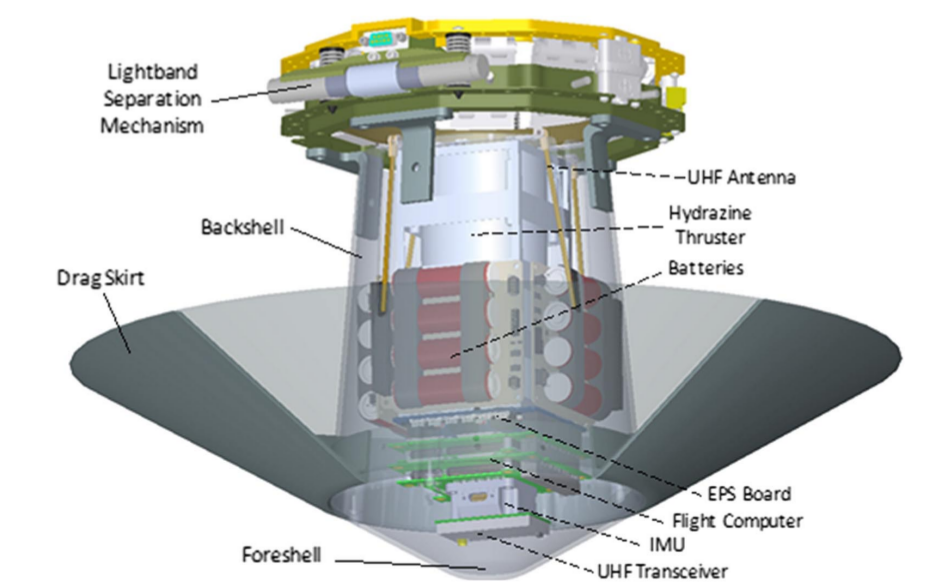
Image credit: M.S.Werner and R.D.Braun
[2]:
from AMAT.planet import Planet
from AMAT.vehicle import Vehicle
[3]:
import numpy as np
from scipy import interpolate
import pandas as pd

import matplotlib.pyplot as plt
from matplotlib import rcParams
[4]:
planet = Planet('MARS')
planet.loadAtmosphereModel('../atmdata/Mars/mars-gram-avg.dat', 0 , 1 ,2, 3)
planet.h_skip = 150.0E3
[5]:
# Set up two vehicle objects, one for 450 km circular, one for 1-sol orbit
vehicle1=Vehicle('MarsSmallSat1', 25.97, 66.4, 0.0, np.pi*0.25**2, 0.0, 0.0563, planet)
vehicle2=Vehicle('MarsSmallSat2', 25.97, 66.4, 0.0, np.pi*0.25**2, 0.0, 0.0563, planet)

vehicle1.setInitialState(150.0,0.0,0.0,5.74,0.0,-5.00,0.0,0.0)
vehicle2.setInitialState(150.0,0.0,0.0,5.74,0.0,-5.00,0.0,0.0)

vehicle1.setSolverParams(1E-6)
vehicle2.setSolverParams(1E-6)

vehicle1.setDragModulationVehicleParams(66.4,4.72)
vehicle2.setDragModulationVehicleParams(66.4,4.72)
First, find the corridor bounds to select a target nominal EFPA for a nominal Mars atmosphere.
[6]:
underShootLimit, exitflag_us = vehicle1.findUnderShootLimitD(2400.0, 0.1, -30.0,-2.0, 1E-10, 450.0)
overShootLimit , exitflag_os = vehicle1.findOverShootLimitD(2400.0, 0.1, -30.0,-2.0, 1E-10,  450.0)

print("450 km circ.")
print("----------------")
print(underShootLimit, exitflag_us)
print(overShootLimit,  exitflag_os)
print("----------------")
underShootLimit, exitflag_us = vehicle2.findUnderShootLimitD(2400.0, 0.1, -30.0,-2.0, 1E-10, 33000.0)
overShootLimit , exitflag_os = vehicle2.findOverShootLimitD(2400.0, 0.1, -30.0,-2.0,  1E-10,  33000.0)

print("1 sol.")
print("----------------")
print(underShootLimit, exitflag_us)
print(overShootLimit,  exitflag_os)
print("----------------")
450 km circ.
----------------
-12.472027218049334 1.0
-11.777824826203869 1.0
----------------
1 sol.
----------------
-12.142672350550129 1.0
-11.459108593211567 1.0
----------------
It is good practice to see how these corridor bounds vary with minimum, average, and maximum density atmospheres. We will check how much these corridor bounds change using +/- 3-sigma bounds from Mars GRAM output files.
Load three density profiles for minimum, average, and maximum scenarios from a GRAM output file.
[7]:
ATM_height, ATM_density_low, ATM_density_avg, ATM_density_high, ATM_density_pert = planet.loadMonteCarloDensityFile2('../atmdata/Mars/LAT00N.txt', 0, 1, 2, 3, 4, heightInKmFlag=True)
density_int_low = planet.loadAtmosphereModel5(ATM_height, ATM_density_low, ATM_density_avg, ATM_density_high, ATM_density_pert, -3.0, 156, 200)
density_int_avg = planet.loadAtmosphereModel5(ATM_height, ATM_density_low, ATM_density_avg, ATM_density_high, ATM_density_pert,  0.0, 156, 200)
density_int_hig = planet.loadAtmosphereModel5(ATM_height, ATM_density_low, ATM_density_avg, ATM_density_high, ATM_density_pert, +3.0, 156, 200)
Set the planet density_int attribute to density_int_low
[8]:
planet.density_int = density_int_low
Compute the corridor bounds for low density atmosphere.
[9]:
underShootLimit, exitflag_us =  vehicle1.findUnderShootLimitD(2400.0, 0.1, -30.0,-2.0, 1E-10, 450.0)
overShootLimit , exitflag_os =  vehicle1.findOverShootLimitD(2400.0, 0.1, -30.0,-2.0, 1E-10,  450.0)

print("450 km circ.")
print("----------------")
print(underShootLimit, exitflag_us)
print(overShootLimit,  exitflag_os)
print("----------------")

underShootLimit, exitflag_us =  vehicle2.findUnderShootLimitD(2400.0, 0.1, -30.0,-2.0, 1E-10, 33000.0)
overShootLimit , exitflag_os =  vehicle2.findOverShootLimitD(2400.0, 0.1, -30.0,-2.0, 1E-10,  33000.0)
print("1-sol.")
print("----------------")
print(underShootLimit, exitflag_us)
print(overShootLimit,  exitflag_os)
print("----------------")
/home/athul/anaconda3/lib/python3.7/site-packages/AMAT-2.1.2-py3.7.egg/AMAT/vehicle.py:504: RuntimeWarning: invalid value encountered in sqrt
  ans[:]  = 1.8980E-8 * (rho_vec[:]/self.RN)**0.5 * v[:]**3.0
450 km circ.
----------------
-12.605845816528017 1.0
-11.993464708328247 1.0
----------------
1-sol.
----------------
-12.326484654251544 1.0
-11.651159566965362 1.0
----------------
Repeat for average and maximum density atmospheres.
[10]:
planet.density_int = density_int_avg
[11]:
underShootLimit, exitflag_us =  vehicle1.findUnderShootLimitD(2400.0, 0.1, -30.0,-2.0, 1E-10, 450.0)
overShootLimit , exitflag_os =  vehicle1.findOverShootLimitD(2400.0, 0.1, -30.0,-2.0, 1E-10,  450.0)

print("450 km circ.")
print("----------------")
print(underShootLimit, exitflag_us)
print(overShootLimit,  exitflag_os)
print("----------------")

underShootLimit, exitflag_us =  vehicle2.findUnderShootLimitD(2400.0, 0.1, -30.0,-2.0, 1E-10, 33000.0)
overShootLimit , exitflag_os =  vehicle2.findOverShootLimitD(2400.0, 0.1, -30.0,-2.0, 1E-10,  33000.0)
print("1-sol.")
print("----------------")
print(underShootLimit, exitflag_us)
print(overShootLimit,  exitflag_os)
print("----------------")
450 km circ.
----------------
-12.545852635754272 1.0
-11.894532441678166 1.0
----------------
1-sol.
----------------
-12.250274132129562 1.0
-11.517179594695335 1.0
----------------
[12]:
planet.density_int = density_int_hig
[13]:
underShootLimit, exitflag_us =  vehicle1.findUnderShootLimitD(2400.0, 0.1, -30.0,-2.0, 1E-10, 450.0)
overShootLimit , exitflag_os =  vehicle1.findOverShootLimitD(2400.0, 0.1, -30.0,-2.0, 1E-10,  450.0)

print("450 km circ.")
print("----------------")
print(underShootLimit, exitflag_us)
print(overShootLimit,  exitflag_os)
print("----------------")

underShootLimit, exitflag_us =  vehicle2.findUnderShootLimitD(2400.0, 0.1, -30.0,-2.0, 1E-10, 33000.0)
overShootLimit , exitflag_os =  vehicle2.findOverShootLimitD(2400.0, 0.1, -30.0,-2.0, 1E-10,  33000.0)
print("1-sol.")
print("----------------")
print(underShootLimit, exitflag_us)
print(overShootLimit,  exitflag_os)
print("----------------")
450 km circ.
----------------
-12.486791579358396 1.0
-11.79002801637398 1.0
----------------
1-sol.
----------------
-12.178909841590212 1.0
-11.394518235101714 1.0
----------------
The above numbers indicate that corridor bounds do not vary that much with atmospheric variations. The corridor is approximately 0.70 deg wide for both target orbits.
[14]:
12.47 - 11.77
[14]:
0.7000000000000011
[15]:
12.14 - 11.45
[15]:
0.6900000000000013
The mid-corridor is typically a good place to start. We will use the mean of the corridor bounds for the average atmosphere.
[16]:
0.5*(-12.47-11.77) # 450 km
[16]:
-12.120000000000001
[17]:
0.5*(-12.14-11.45) # 1-sol
[17]:
-11.795
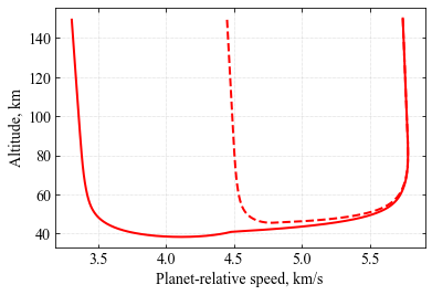
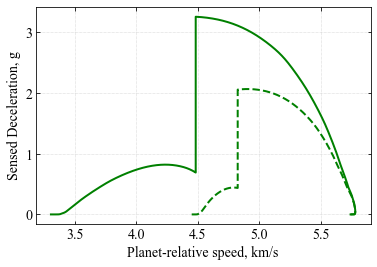
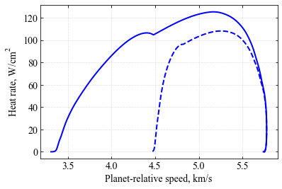
We will propogate a nominal guided trajectory to reproduce Fig. 10 from the paper.
[18]:
planet.loadAtmosphereModel('../atmdata/Mars/mars-gram-avg.dat', 0 , 1 ,2, 3)
[19]:
# Set planet.h_low to 10 km, if vehicle dips below this level
# trajctory is terminated.
planet.h_low=10.0E3

# Set target orbit = 450 km x 450 km, tolerance = 50 km
vehicle1.setTargetOrbitParams(450.0, 450.0, 20.0)
vehicle2.setTargetOrbitParams(450.0, 33000.0, 20.0)

# Set entry phase parameters
# v_switch_kms = 2.0, lowAlt_km = 20.0,
# numPoints_lowAlt = 101, hdot_threshold = -200.0 m/s.
# These are somewhat arbitary based on experience.
vehicle1.setDragEntryPhaseParams(2.0, 20.0, 101, -200.0)
vehicle2.setDragEntryPhaseParams(2.0, 20.0, 101, -200.0)

# Set beta_1 and beta_ratio
vehicle1.setDragModulationVehicleParams(66.4,4.72)
vehicle2.setDragModulationVehicleParams(66.4,4.72)

# Set vehicle initial state
vehicle1.setInitialState(150.0,0.0,0.0,5.74,0.0,-12.12,0.0,0.0)
vehicle2.setInitialState(150.0,0.0,0.0,5.74,0.0,-11.80,0.0,0.0)
[20]:
# Propogate a single vehicle trajectory
vehicle1.propogateGuidedEntryD(1.0,1.0,0.1,2400.0)
vehicle2.propogateGuidedEntryD(1.0,1.0,0.1,2400.0)
[21]:
plt.figure(figsize=(6,4))
plt.rc('font',family='Times New Roman')
params = {'mathtext.default': 'regular' }
plt.rcParams.update(params)
plt.plot(vehicle1.v_kms_full, vehicle1.h_km_full, 'r-', linewidth=2.0)
plt.plot(vehicle2.v_kms_full, vehicle2.h_km_full, 'r--', linewidth=2.0)

plt.xlabel('Planet-relative speed, km/s',fontsize=14)
plt.ylabel('Altitude, km',fontsize=14)
ax=plt.gca()
ax.tick_params(direction='in')
ax.yaxis.set_ticks_position('both')
ax.xaxis.set_ticks_position('both')
ax.tick_params(axis='x',labelsize=14)
ax.tick_params(axis='y',labelsize=14)
plt.grid(linestyle='dotted', linewidth=0.5)

plt.savefig('../plots/werner-smallsat-nominal-altitude-speed-mars.png',bbox_inches='tight')
plt.savefig('../plots/werner-smallsat-nominal-altitude-speed-mars.pdf', dpi=300,bbox_inches='tight')
plt.savefig('../plots/werner-smallsat-nominal-altitude-speed-mars.eps', dpi=300,bbox_inches='tight')

plt.show()
[22]:
plt.figure(figsize=(6,4))
plt.rc('font',family='Times New Roman')
params = {'mathtext.default': 'regular' }
plt.rcParams.update(params)
plt.plot(vehicle1.v_kms_full, vehicle1.acc_net_g_full, 'g-', linewidth=2.0)
plt.plot(vehicle2.v_kms_full, vehicle2.acc_net_g_full, 'g--', linewidth=2.0)

plt.xlabel('Planet-relative speed, km/s',fontsize=14)
plt.ylabel('Sensed Deceleration, g',fontsize=14)
ax=plt.gca()
ax.tick_params(direction='in')
ax.yaxis.set_ticks_position('both')
ax.xaxis.set_ticks_position('both')
ax.tick_params(axis='x',labelsize=14)
ax.tick_params(axis='y',labelsize=14)
plt.grid(linestyle='dotted', linewidth=0.5)

plt.savefig('../plots/werner-smallsat-nominal-speed-decel-mars.png',bbox_inches='tight')
plt.savefig('../plots/werner-smallsat-nominal-speed-decel-mars.pdf', dpi=300,bbox_inches='tight')
plt.savefig('../plots/werner-smallsat-nominal-speed-decel-mars.eps', dpi=300,bbox_inches='tight')

plt.show()
[23]:
plt.figure(figsize=(6,4))
plt.rc('font',family='Times New Roman')
params = {'mathtext.default': 'regular' }
plt.rcParams.update(params)
plt.plot(vehicle1.v_kms_full, vehicle1.q_stag_total_full, 'b-', linewidth=2.0)
plt.plot(vehicle2.v_kms_full, vehicle2.q_stag_total_full, 'b--', linewidth=2.0)


plt.xlabel('Planet-relative speed, km/s',fontsize=14)
plt.ylabel('Heat rate, '+r'$W/cm^2$',fontsize=14)
ax=plt.gca()
ax.tick_params(direction='in')
ax.yaxis.set_ticks_position('both')
ax.xaxis.set_ticks_position('both')
ax.tick_params(axis='x',labelsize=14)
ax.tick_params(axis='y',labelsize=14)
plt.grid(linestyle='dotted', linewidth=0.5)

plt.savefig('../plots/werner-smallsat-nominal-speed-heat-mars.png',bbox_inches='tight')
plt.savefig('../plots/werner-smallsat-nominal-speed-heat-mars.pdf', dpi=300,bbox_inches='tight')
plt.savefig('../plots/werner-smallsat-nominal-speed-heat-mars.eps', dpi=300,bbox_inches='tight')

plt.show()
[24]:
vehicle1.terminal_apoapsis
[24]:
612.6745425743503
[25]:
vehicle2.terminal_apoapsis
[25]:
32890.38040256599