Example - 55 - Titan Aerocapture Systems Study - Part 1
This examples reproduces results from Way, Powell et al., Aerocapture Simulation and Performance for the Titan Explorer Mission, 39th AIAA/ASME/SAE/ASEE Joint Propulsion Conference and Exhibit 20-23 July 2003, Huntsville, Alabama. https://doi.org/10.2514/6.2003-4951
[1]:
from IPython.display import Image
Image(filename='../plots/titan-aerocapture-systems.png', width=500)
[1]:

Image credit: Lockwood et al.
[2]:
from AMAT.planet import Planet
from AMAT.vehicle import Vehicle
[3]:
import numpy as np
from scipy import interpolate
import pandas as pd

import matplotlib.pyplot as plt
from matplotlib import rcParams
[4]:
planet = Planet('TITAN')
planet.loadAtmosphereModel('../atmdata/Titan/titan-gram-avg.dat', 0 , 1 ,2, 3)
planet.h_skip = 1000.0E3
[5]:
vehicle=Vehicle('TitanAC', 818.0, 90.0, 0.25, np.pi*0.25*3.75**2, 0.0, 0.91, planet)
vehicle.setInitialState(1000.0,0.0,0.0,6.5,0.0,-25.00,0.0,0.0)
vehicle.setSolverParams(1E-6)
First, find the corridor bounds to select a target nominal EFPA for a nominal Mars atmosphere.
[7]:
underShootLimit, exitflag_us = vehicle.findUnderShootLimit(60.0*60.0, 1.0, -50.0,-5.0, 1E-10,  1700.0)
overShootLimit , exitflag_os = vehicle.findOverShootLimit(60.0*60.0,  1.0, -50.0,-5.0, 1E-10,  1700.0)

print("Corridor bounds for nominal atmosphere.")
print("----------------")
print(underShootLimit, exitflag_us)
print(overShootLimit,  exitflag_os)
print("----------------")
Corridor bounds for nominal atmosphere.
----------------
-37.83097717905548 1.0
-34.28877212249972 1.0
----------------
It is good practice to see how these corridor bounds vary with minimum, average, and maximum density atmospheres. We will check how much these corridor bounds change using +/- 3-sigma bounds from Titan GRAM output files.
Load three density profiles for minimum, average, and maximum scenarios from a GRAM output file.
[9]:
ATM_height1, ATM_density_low1, ATM_density_avg1, ATM_density_high1, ATM_density_pert1 = planet.loadMonteCarloDensityFile2('../atmdata/Titan/FMINMAX-10.txt', 0, 1, 2, 3, 4, heightInKmFlag=True)
ATM_height2, ATM_density_low2, ATM_density_avg2, ATM_density_high2, ATM_density_pert2 = planet.loadMonteCarloDensityFile2('../atmdata/Titan/FMINMAX+00.txt', 0, 1, 2, 3, 4, heightInKmFlag=True)
ATM_height3, ATM_density_low3, ATM_density_avg3, ATM_density_high3, ATM_density_pert3 = planet.loadMonteCarloDensityFile2('../atmdata/Titan/FMINMAX+10.txt', 0, 1, 2, 3, 4, heightInKmFlag=True)


density_int_low = planet.loadAtmosphereModel5(ATM_height1, ATM_density_low1, ATM_density_avg1, ATM_density_high1, ATM_density_pert1, -3.0, 201, 1)
density_int_avg = planet.loadAtmosphereModel5(ATM_height2, ATM_density_low2, ATM_density_avg2, ATM_density_high2, ATM_density_pert2,  0.0, 201, 1)
density_int_hig = planet.loadAtmosphereModel5(ATM_height3, ATM_density_low3, ATM_density_avg3, ATM_density_high3, ATM_density_pert3, +3.0, 201, 1)
Set the planet density_int attribute to density_int_low
[10]:
planet.density_int = density_int_low
Compute the corridor bounds for low density atmosphere.
[11]:
underShootLimit, exitflag_us = vehicle.findUnderShootLimit(60.0*60.0, 1.0, -50.0,-5.0, 1E-10,  1700.0)
overShootLimit , exitflag_os = vehicle.findOverShootLimit(60.0*60.0,  1.0, -50.0,-5.0, 1E-10,  1700.0)

print("Low density atmosphere corridor bounds.")
print("----------------")
print(underShootLimit, exitflag_us)
print(overShootLimit,  exitflag_os)
print("----------------")
Low density atmosphere corridor bounds.
----------------
-38.47725151913437 1.0
-35.15044797081828 1.0
----------------
Repeat for average and maximum density atmospheres.
[13]:
planet.density_int = density_int_avg
[14]:
underShootLimit, exitflag_us = vehicle.findUnderShootLimit(60.0*60.0, 1.0, -50.0,-5.0, 1E-10,  1700.0)
overShootLimit , exitflag_os = vehicle.findOverShootLimit(60.0*60.0,  1.0, -50.0,-5.0, 1E-10,  1700.0)

print("Average density atmosphere corridor bounds.")
print("----------------")
print(underShootLimit, exitflag_us)
print(overShootLimit,  exitflag_os)
print("----------------")
Average density atmosphere corridor bounds.
----------------
-37.86181146377203 1.0
-34.38959433911805 1.0
----------------
[15]:
planet.density_int = density_int_hig
[16]:
underShootLimit, exitflag_us = vehicle.findUnderShootLimit(60.0*60.0, 1.0, -50.0,-5.0, 1E-10,  1700.0)
overShootLimit , exitflag_os = vehicle.findOverShootLimit(60.0*60.0,  1.0, -50.0,-5.0, 1E-10,  1700.0)

print("High density atmosphere corridor bounds.")
print("----------------")
print(underShootLimit, exitflag_us)
print(overShootLimit,  exitflag_os)
print("----------------")
High density atmosphere corridor bounds.
----------------
-37.287857468882066 1.0
-33.65637210436944 1.0
----------------
The corridor is approximately 3.5 deg wide for the nominal atmosphere.
[17]:
37.86 - 34.39
[17]:
3.469999999999999
The mid-corridor is typically a good place to start. We will use the mean of the corridor bounds for the average atmosphere.
[18]:
0.5*(-37.86 - 34.39)
[18]:
-36.125
We will propogate a bounding trajectories to illustrate full lift up and full lift down aerocapture trajectories at Titan using this vehicle.
[21]:
planet.density_int = density_int_avg
[27]:
# Reset initial conditions and propogate overshoot trajectory
vehicle.setInitialState(1000.0,0.0,0.0,6.5,0.0,-34.38959433911805,0.0,0.0)
vehicle.propogateEntry (60.0*60.0,1.0,180.0)
# Extract and save variables to plot
t_min_os = vehicle.t_minc
h_km_os = vehicle.h_kmc
acc_net_g_os = vehicle.acc_net_g
q_stag_con_os = vehicle.q_stag_con
q_stag_rad_os = vehicle.q_stag_rad
# Reset initial conditions and propogate undershoot trajectory
vehicle.setInitialState(1000.0,0.0,0.0,6.5,0.0,-37.86181146377203,0.0,0.0)
vehicle.propogateEntry (60.0*60.0,1.0,0.0)
# Extract and save variable to plot
t_min_us = vehicle.t_minc
h_km_us = vehicle.h_kmc
acc_net_g_us = vehicle.acc_net_g
q_stag_con_us = vehicle.q_stag_con
q_stag_rad_us = vehicle.q_stag_rad
'''
Create fig #1 - altitude history of aerocapture maneuver
'''
fig = plt.figure()
fig.set_size_inches([6.5,6.5])
plt.rc('font',family='Times New Roman')
params = {'mathtext.default': 'regular' }
plt.rcParams.update(params)
plt.plot(t_min_os , h_km_os, linestyle='solid' , color='xkcd:blue',linewidth=2.0, label='Overshoot')
plt.plot(t_min_us , h_km_us, linestyle='solid' , color='xkcd:green',linewidth=2.0, label='Undershoot')
plt.xlabel('Time, min',fontsize=14)
plt.ylabel("Altitude, km",fontsize=14)
ax = plt.gca()
ax.tick_params(direction='in')
ax.yaxis.set_ticks_position('both')
ax.xaxis.set_ticks_position('both')
plt.tick_params(direction='in')
plt.tick_params(axis='x',labelsize=14)
plt.tick_params(axis='y',labelsize=14)
plt.legend(loc='lower right', fontsize=14)
plt.savefig('../plots/titan-systems-altitude.png',bbox_inches='tight')
plt.savefig('../plots/titan-systems-altitude.pdf', dpi=300,bbox_inches='tight')
plt.savefig('../plots/titan-systems-altitude.eps', dpi=300,bbox_inches='tight')
plt.show()
fig = plt.figure()
fig.set_size_inches([6.5,6.5])
plt.rc('font',family='Times New Roman')
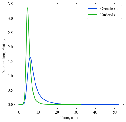
plt.plot(t_min_os , acc_net_g_os, linestyle='solid' , color='xkcd:blue',linewidth=2.0, label='Overshoot')
plt.plot(t_min_us , acc_net_g_us, linestyle='solid' , color='xkcd:green',linewidth=2.0, label='Undershoot')
plt.xlabel('Time, min',fontsize=14)
plt.ylabel("Deceleration, Earth g",fontsize=14)
ax = plt.gca()
ax.tick_params(direction='in')
ax.yaxis.set_ticks_position('both')
ax.xaxis.set_ticks_position('both')
plt.tick_params(direction='in')
plt.tick_params(axis='x',labelsize=14)
plt.tick_params(axis='y',labelsize=14)
plt.legend(loc='upper right', fontsize=14)
plt.savefig('../plots/titan-systems-deceleration.png',bbox_inches='tight')
plt.savefig('../plots/titan-systems-deceleration.pdf', dpi=300,bbox_inches='tight')
plt.savefig('../plots/titan-systems-deceleration.eps', dpi=300,bbox_inches='tight')
plt.show()
fig = plt.figure()
fig.set_size_inches([6.5,6.5])
plt.rc('font',family='Times New Roman')
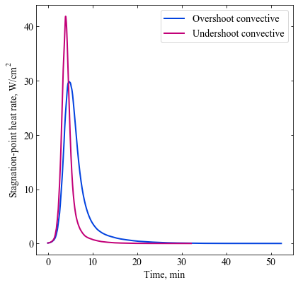
plt.plot(t_min_os , q_stag_con_os, linestyle='solid' , color='xkcd:blue',linewidth=2.0, label='Overshoot convective')
plt.plot(t_min_us , q_stag_con_us, linestyle='solid' , color='xkcd:magenta',linewidth=2.0, label='Undershoot convective')
plt.xlabel('Time, min',fontsize=14)
plt.ylabel("Stagnation-point heat rate, "+r'$W/cm^2$',fontsize=14)
ax = plt.gca()
ax.tick_params(direction='in')
ax.yaxis.set_ticks_position('both')
ax.xaxis.set_ticks_position('both')
plt.tick_params(direction='in')
plt.tick_params(axis='x',labelsize=14)
plt.tick_params(axis='y',labelsize=14)
plt.legend(loc='upper right', fontsize=14)
plt.savefig('../plots/titan-systems-heating.png',bbox_inches='tight')
plt.savefig('../plots/titan-systems-heating.pdf', dpi=300,bbox_inches='tight')
plt.savefig('../plots/titan-systems-heating.eps', dpi=300,bbox_inches='tight')
plt.show()
The PostScript backend does not support transparency; partially transparent artists will be rendered opaque.
The PostScript backend does not support transparency; partially transparent artists will be rendered opaque.
The PostScript backend does not support transparency; partially transparent artists will be rendered opaque.
The PostScript backend does not support transparency; partially transparent artists will be rendered opaque.

The PostScript backend does not support transparency; partially transparent artists will be rendered opaque.
The PostScript backend does not support transparency; partially transparent artists will be rendered opaque.
The PostScript backend does not support transparency; partially transparent artists will be rendered opaque.
The PostScript backend does not support transparency; partially transparent artists will be rendered opaque.
The PostScript backend does not support transparency; partially transparent artists will be rendered opaque.
The PostScript backend does not support transparency; partially transparent artists will be rendered opaque.
The PostScript backend does not support transparency; partially transparent artists will be rendered opaque.
The PostScript backend does not support transparency; partially transparent artists will be rendered opaque.