Example - 63 - Locus of approach trajectories for constant inertial EFPA

In this example, we illustrate the locus of approach trajectories for constant inertial entry-flight path angle (EFPA) from an interplanetary trajectory.

Note: This example requires Mayavi for visualization and requires the following packages to be to be installed in your virtual env: pyqt5, vtk, mayavi.

Note: For the 3D viz, tt is recommended that you run this example by running the python file using: python example-63-locus-of-approach-trajectories.py from your virtual env terminal instead of this Jupyter Notebook. If you use this Jupyter Notebook, then you need to have the following additional packages installed ipywidgets and ipyevents, and must do jupyter nbextension install --py mayavi --user before you start the notebook.

from mayavi import mlab
mlab.init_notebook(backend='ipy')

import numpy as np

from tvtk.tools import visual
from AMAT.approach import Approach

Notebook initialized with ipy backend.

def Arrow_From_A_to_B(x1, y1, z1, x2, y2, z2):
    ar1 = visual.arrow(x=x1, y=y1, z=z1)
    ar1.length_cone = 0.4

    arrow_length = np.sqrt((x2 - x1) ** 2 + (y2 - y1) ** 2 + (z2 - z1) ** 2)
    ar1.actor.scale = [arrow_length, arrow_length, arrow_length]
    ar1.pos = ar1.pos / arrow_length
    ar1.axis = [x2 - x1, y2 - y1, z2 - z1]
    return ar1

Compute approach trajectories for psi = [0, 2pi]

u = np.linspace(0, 2 * np.pi, 100)
v = np.linspace(0, np.pi, 100)
x = 1 * np.outer(np.cos(u), np.sin(v))
y = 1 * np.outer(np.sin(u), np.sin(v))
z = 1 * np.outer(np.ones(np.size(u)), np.cos(v))

x1 = 1.040381198513972 * np.outer(np.cos(u), np.sin(v))
y1 = 1.040381198513972 * np.outer(np.sin(u), np.sin(v))
z1 = 1.040381198513972 * np.outer(np.ones(np.size(u)), np.cos(v))

x_ring_1 = 1.1 * np.cos(u)
y_ring_1 = 1.1 * np.sin(u)
z_ring_1 = 0.0 * np.cos(u)

x_ring_2 = 1.2 * np.cos(u)
y_ring_2 = 1.2 * np.sin(u)
z_ring_2 = 0.0 * np.cos(u)

mlab.figure(bgcolor=(0, 0, 0))
s1 = mlab.mesh(x, y, z, color=(0, 0, 1))
s2 = mlab.mesh(x1, y1, z1, color=(0, 0, 1), opacity=0.3)
r1 = mlab.plot3d(x_ring_1, y_ring_1, z_ring_1, color=(1, 1, 1), line_width=1, tube_radius=None)
r2 = mlab.plot3d(x_ring_2, y_ring_2, z_ring_2, color=(1, 1, 1), line_width=1, tube_radius=None)

for psi in np.linspace(0, 2 * np.pi, 31):
    probe = Approach("NEPTUNE",
                     v_inf_vec_icrf_kms=np.array([17.78952518, 8.62038536, 3.15801163]),
                     rp=(24622 + 400) * 1e3, psi=psi,
                     is_entrySystem=True, h_EI=1000e3)

    theta_star_arr_probe1 = np.linspace(-1.7, probe.theta_star_entry, 101)
    pos_vec_bi_arr_probe1 = probe.pos_vec_bi(theta_star_arr_probe1) / 24622e3

    x_arr_probe = pos_vec_bi_arr_probe1[0][:]
    y_arr_probe = pos_vec_bi_arr_probe1[1][:]
    z_arr_probe = pos_vec_bi_arr_probe1[2][:]

    mlab.plot3d(x_arr_probe, y_arr_probe, z_arr_probe, color=(1, 0, 0), line_width=3, tube_radius=None)

    if psi == 0:
        mlab.plot3d([0, 2 * probe.v_inf_vec_bi_unit[0]],
                    [0, 2 * probe.v_inf_vec_bi_unit[1]],
                    [0, 2 * probe.v_inf_vec_bi_unit[2]])

mlab.show()

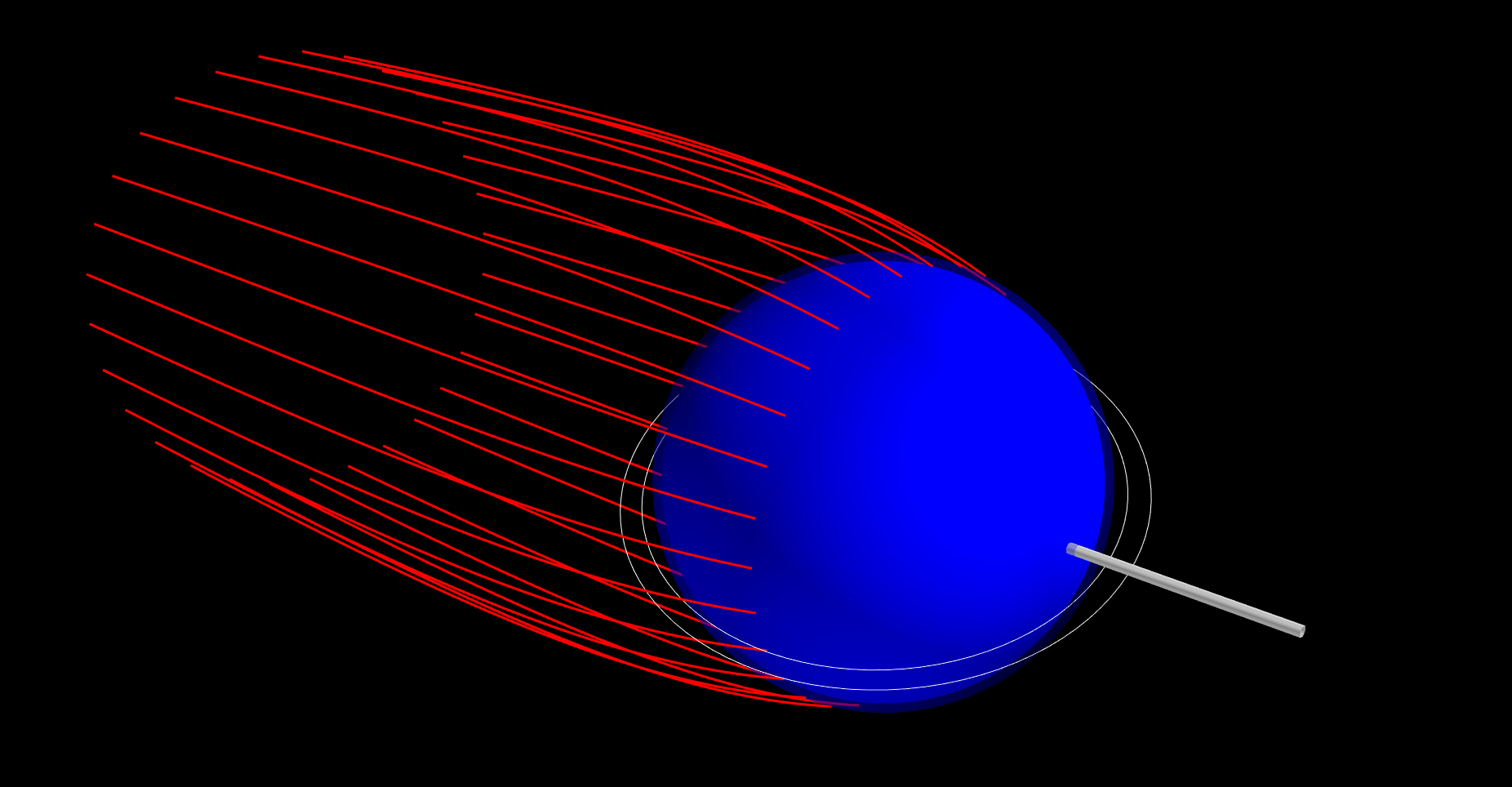
Plot the locus of approach trajectories

from IPython.display import Image
Image(filename="../plots/example-63-locus-of-approach-trajectories.png", width=800)