Example - 49 - Earth SmallSat Aerocapture Demonstration - Part 1

This examples reproduces results from M.S.Werner and R.D.Braun, Mission Design and Performance Analysis of a Smallsat Aerocapture Flight Test, Journal of Spacecraft and Rockets, DOI: 10.2514/1.A33997.

from IPython.display import Image
Image(filename='../plots/werner-smallsat.png', width=500)

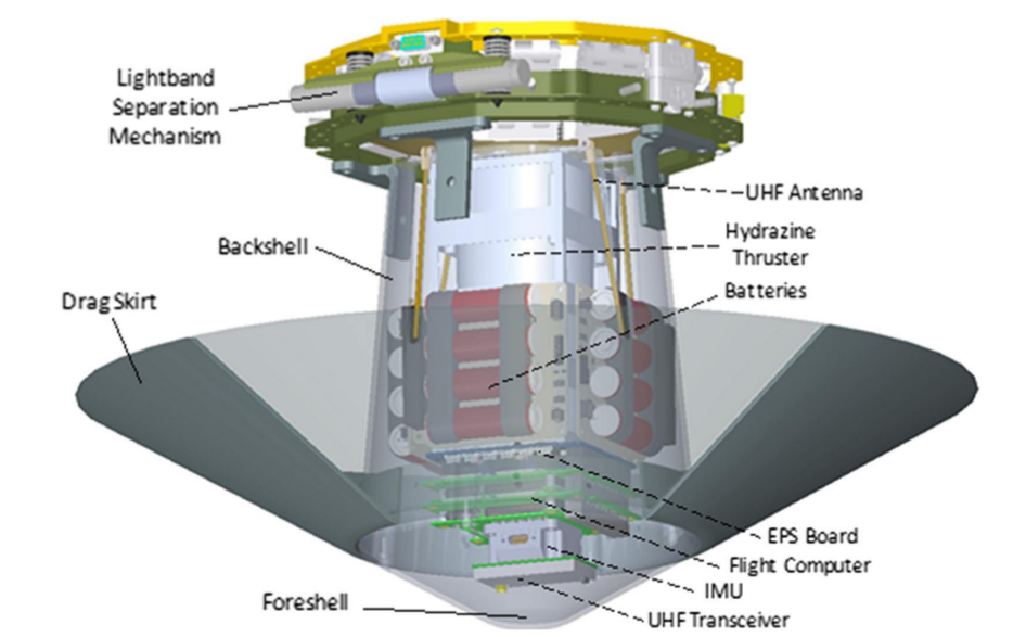
Image credit: M.S.Werner and R.D.Braun

from AMAT.planet import Planet
from AMAT.vehicle import Vehicle

import numpy as np
from scipy import interpolate
import pandas as pd

import matplotlib.pyplot as plt
from matplotlib import rcParams

planet = Planet('EARTH')
planet.loadAtmosphereModel('../atmdata/Earth/earth-gram-avg.dat', 0 , 1 ,2, 3)
planet.h_skip = 125.0E3

vehicle=Vehicle('EarthSmallSat', 25.97, 66.4, 0.0, np.pi*0.25**2, 0.0, 0.0563, planet)
vehicle.setInitialState(125.0,0.0,0.0,9.8,0.0,-5.00,0.0,0.0)
vehicle.setSolverParams(1E-6)
vehicle.setDragModulationVehicleParams(66.4,4.72)

First, find the corridor bounds to select a target nominal EFPA for a nominal Earth atmosphere.

underShootLimit, exitflag_us = vehicle.findUnderShootLimitD(2400.0, 0.1, -30.0,-2.0, 1E-10, 1760.0)
overShootLimit , exitflag_os =  vehicle.findOverShootLimitD(2400.0, 0.1, -30.0,-2.0, 1E-10, 1760.0)

print(underShootLimit, exitflag_us)
print(overShootLimit,  exitflag_os)

-5.141069082768809 1.0
-4.649618244053272 1.0

It is good practice to see how these corridor bounds vary with minimum, average, and maximum density atmospheres. We will check how much these corridor bounds change using +/- 3-sigma bounds from EARTH GRAM output files.

Load three density profiles for minimum, average, and maximum scenarios from a GRAM output file.

ATM_height, ATM_density_low, ATM_density_avg, ATM_density_high, ATM_density_pert = planet.loadMonteCarloDensityFile3('../atmdata/Earth/LAT00N.txt', 1, 4, 14, 9, heightInKmFlag=True)
density_int_low = planet.loadAtmosphereModel5(ATM_height, ATM_density_low, ATM_density_avg, ATM_density_high, ATM_density_pert, -3.0, 141, 200)
density_int_avg = planet.loadAtmosphereModel5(ATM_height, ATM_density_low, ATM_density_avg, ATM_density_high, ATM_density_pert,  0.0, 141, 200)
density_int_hig = planet.loadAtmosphereModel5(ATM_height, ATM_density_low, ATM_density_avg, ATM_density_high, ATM_density_pert, +3.0, 141, 200)

Set the planet density_int attribute to density_int_low

planet.density_int = density_int_low

Compute the corridor bounds for low density atmosphere.

underShootLimit, exitflag_us = vehicle.findUnderShootLimitD(2400.0, 0.1, -30.0,-2.0, 1E-10, 1760.0)
overShootLimit , exitflag_os =  vehicle.findOverShootLimitD(2400.0, 0.1, -30.0,-2.0, 1E-10, 1760.0)

print(underShootLimit, exitflag_us)
print(overShootLimit,  exitflag_os)

-5.2014596410954255 1.0
-4.72837330459879 1.0

Repeat for average and maximum density atmospheres.

planet.density_int = density_int_avg

underShootLimit, exitflag_us = vehicle.findUnderShootLimitD(2400.0, 0.1, -30.0, -2.0, 1E-10, 1760.0)
overShootLimit , exitflag_os =  vehicle.findOverShootLimitD(2400.0, 0.1, -30.0, -2.0, 1E-10, 1760.0)

print(underShootLimit, exitflag_us)
print(overShootLimit,  exitflag_os)

-5.14605522868078 1.0
-4.6526982840077835 1.0

planet.density_int = density_int_hig

underShootLimit, exitflag_us = vehicle.findUnderShootLimitD(2400.0, 0.1, -30.0, -2.0, 1E-10, 1760.0)
overShootLimit , exitflag_os =  vehicle.findOverShootLimitD(2400.0, 0.1, -30.0, -2.0, 1E-10, 1760.0)

print(underShootLimit, exitflag_us)
print(overShootLimit,  exitflag_os)

-5.096641375908803 1.0
-4.5848947728809435 1.0

The above numbers indicate that corridor bounds do not vary that much with atmospheric variations. The corridor is approximately 0.50 deg wide.

5.09-4.58

0.5099999999999998

The mid-corridor is typically a good place to start. We will use the mean of the corridor bounds for the average atmosphere.

0.5*(-4.65-5.15)

-4.9

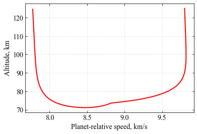
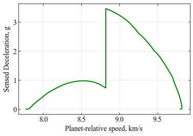
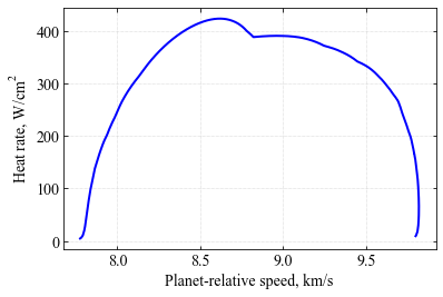
We will propogate a nominal guided trajectory to reproduce Fig. 5 from the paper.

# Set planet.h_low to 10 km, if vehicle dips below this level
# trajctory is terminated.
planet.h_low=10.0E3

# Set target orbit = 180 km x 1760, tolerance = 50 km
vehicle.setTargetOrbitParams(180.0, 1760.0, 50.0)

# Set entry phase parameters
# v_switch_kms = 5.0, lowAlt_km = 50.0,
# numPoints_lowAlt = 101, hdot_threshold = -200.0 m/s.
# These are somewhat arbitary based on experience.
vehicle.setDragEntryPhaseParams(5.0, 50.0, 101, -200.0)

# Set beta_1 and beta_ratio
vehicle.setDragModulationVehicleParams(66.4,4.72)

# Set vehicle initial state
vehicle.setInitialState(125.0,0.0,0.0,9.8,0.0,-4.90,0.0,0.0)

# Propogate a single vehicle trajectory
vehicle.propogateGuidedEntryD(1.0,1.0,0.1,2400.0)

plt.figure(figsize=(6,4))
plt.rc('font',family='Times New Roman')
params = {'mathtext.default': 'regular' }
plt.rcParams.update(params)
plt.plot(vehicle.v_kms_full, vehicle.h_km_full, 'r-', linewidth=2.0)

plt.xlabel('Planet-relative speed, km/s',fontsize=14)
plt.ylabel('Altitude, km',fontsize=14)
ax=plt.gca()
ax.tick_params(direction='in')
ax.yaxis.set_ticks_position('both')
ax.xaxis.set_ticks_position('both')
ax.tick_params(axis='x',labelsize=14)
ax.tick_params(axis='y',labelsize=14)
plt.grid(linestyle='dotted', linewidth=0.5)

plt.savefig('../plots/werner-smallsat-nominal-altitude-speed.png',bbox_inches='tight')
plt.savefig('../plots/werner-smallsat-nominal-altitude-speed.pdf', dpi=300,bbox_inches='tight')
plt.savefig('../plots/werner-smallsat-nominal-altitude-speed.eps', dpi=300,bbox_inches='tight')

plt.show()

plt.figure(figsize=(6,4))
plt.rc('font',family='Times New Roman')
params = {'mathtext.default': 'regular' }
plt.rcParams.update(params)
plt.plot(vehicle.v_kms_full, vehicle.acc_net_g_full, 'g-', linewidth=2.0)


plt.xlabel('Planet-relative speed, km/s',fontsize=14)
plt.ylabel('Sensed Deceleration, g',fontsize=14)
ax=plt.gca()
ax.tick_params(direction='in')
ax.yaxis.set_ticks_position('both')
ax.xaxis.set_ticks_position('both')
ax.tick_params(axis='x',labelsize=14)
ax.tick_params(axis='y',labelsize=14)
plt.grid(linestyle='dotted', linewidth=0.5)

plt.savefig('../plots/werner-smallsat-nominal-speed-decel.png',bbox_inches='tight')
plt.savefig('../plots/werner-smallsat-nominal-speed-decel.pdf', dpi=300,bbox_inches='tight')
plt.savefig('../plots/werner-smallsat-nominal-speed-decel.eps', dpi=300,bbox_inches='tight')

plt.show()

plt.figure(figsize=(6,4))
plt.rc('font',family='Times New Roman')
params = {'mathtext.default': 'regular' }
plt.rcParams.update(params)
plt.plot(vehicle.v_kms_full, vehicle.q_stag_total_full, 'b-', linewidth=2.0)


plt.xlabel('Planet-relative speed, km/s',fontsize=14)
plt.ylabel('Heat rate, '+r'$W/cm^2$',fontsize=14)
ax=plt.gca()
ax.tick_params(direction='in')
ax.yaxis.set_ticks_position('both')
ax.xaxis.set_ticks_position('both')
ax.tick_params(axis='x',labelsize=14)
ax.tick_params(axis='y',labelsize=14)
plt.grid(linestyle='dotted', linewidth=0.5)

plt.savefig('../plots/werner-smallsat-nominal-speed-heat.png',bbox_inches='tight')
plt.savefig('../plots/werner-smallsat-nominal-speed-heat.pdf', dpi=300,bbox_inches='tight')
plt.savefig('../plots/werner-smallsat-nominal-speed-heat.eps', dpi=300,bbox_inches='tight')

plt.show()

vehicle.terminal_apoapsis

1759.9133624138142